1.4 STATE MODEL OF A GENERAL CONTROL SYSTEM
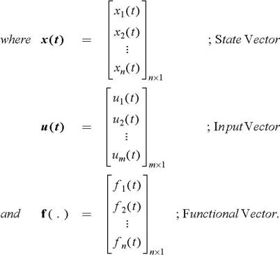
For a general system of Figure 1.1, the state representation can be arranged in the form of n first-order differential equations as
Integrating (1.1), we have
Thus, the n state-variables and, the state of the system can uniquely be determined at any t < t n, provided each state-variable is known at t = t n and all the m control forces are known throughout the interval t 0 to t.
The n differential equations of (1.1) may be written in vector form as
Equation (1.2) is the state equation for time-invariant systems. However, for time-varying systems, the function vector f(.) is dependent on time as well, and the vector equation may be given as
Equation (1.3) is the state equation for time-varying systems.
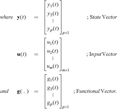
The output y( t) can, in general, be expressed in terms of the state vector x( t) and input vector u( t) as:
For time-invariant systems:
For time-varying systems:
Equations (1.4) and (1.5) are the output equations for time-invariant and time-varying systems, respectively.
The state equations and output equations together constitute the state model of the system. Thus, the state model of a general control system (shown in Figure 1.1) is given by the following equations:
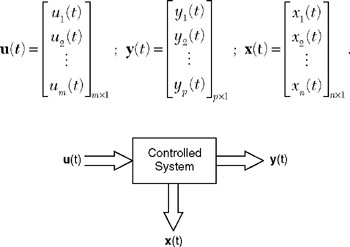 Figure 1.1: Block-diagram representation of a general control system
 For time-invariant systems:
For time-varying systems:

 TABLE OF CONTENTS