Neural Networks for RF and Microwave Design

An electrical engineering textbook on practical applications of artificial intelligence technology methods to solving complex radio-frequency and microwave design problems.
In this section, three conductor microstripline and physics-based MESFET modeling examples are used to compare the performance of various training algorithms for feedforward neural networks namely, the adaptive back propagation, conjugate-gradient, Quasi-Newton, and Levenberg-Marquardt algorithms [2].
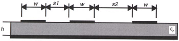
For the microstripline example, there are five input neurons corresponding to conductor width ( w), spacing between conductors ( s 1, s 2), substrate height ( h), and relative permittivity ( ? r), as shown in Figure 4.29. There are six output neurons corresponding to the self-inductance of each conductor ( L 11, L 22, L 33), and the mutual inductance between any two conductors ( L 12, L 23, L 13). A total of 600 training samples and 640 test samples were generated using LINPAR [54]. A three-layer MLP structure with 28 hidden neurons was used, and the training results are shown in Table 4.4. The CPU time was given for a 200 MHz Pentium.
| Training Algorithm | No. of Epochs | Training Error (%) | Avg. Test Error (%) | CPU (in Sec) |
|---|---|---|---|---|
| Adaptive back propagation | 10,755 | 0.224 | 0.252 | 13,724 |
| Conjugate-gradient | 2,169 | 0.415 | 0.473 |