Neural Networks for RF and Microwave Design

An electrical engineering textbook on practical applications of artificial intelligence technology methods to solving complex radio-frequency and microwave design problems.
In this section, different training techniques are compared. First, based on the ability to find local and global minimums, we make the following observations. Conjugate-gradient, Quasi-Newton, and Levenberg-Marquardt algorithms converge to a local minimum that is nearest to the initial guess. The stochastic BP and simplex methods may escape the nearest local minimum, but they'll ultimately end up in some other local minimum. Genetic algorithms and simulated annealing both have the ability to find the global minimum.
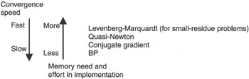
Second, training techniques are compared on the basis of computation speed and memory requirements, and are ranked as shown in Figure 4.28. A detailed comparison of the training algorithms is also presented in Table 4.3.
| Part A | ||||
|---|---|---|---|---|
| Training Algorithm | Convergence Speed (Number of Epochs) | CPU/Epoch | Total CPU (Small Neural Network) | Total CPU (Large Neural Network) |
| Levenberg-Marquardt | Few | LU of a large matrix | Small | Huge |
| Quasi-Newton | Few | Matrix/Vector product | Small | Huge |
| Conjugate-gradient | Medium | Vector/Vector product | Small | Large |
| Back propagation | Large | Scalar operations | Large | Large |
| Simplex method | Large | Scalar operations | Large | Large |
| Genetic algorithm/Simulated Annealing | Very Large | Scalar operations | Large | Huge |
| Part B | |||
|---|---|---|---|
| Training Algorithm | Ease of Implementation | Memory Requirement | Likelihood of Reaching Global Minimum |
| Levenberg-Marquardt Quasi-Newton Conjugate-gradient | Needs effort | Matrix Matrix Vectors | Depends on initial guess of the neural network weight parameters |
| Back propagation | Easiest | Small vectors | Possible |
| Simplex method | Easy | Vectors |