Applied Electromagnetics Using QuickField™ and MATLAB® is intended
as an introductory level textbook for teaching computer-based electricity,
magnetism and multiphysics. The text is easily accessible to advanced
undergraduates and beginning graduate students in physics and engineering.
Many exercises and demonstrations may be implemented using QuickField and
MATLAB in a traditional introductory level physics course. This second audience
will benefit from the visualization of electric and magnetic field distributions
and force calculations without a working knowledge of the finite element
method or potential theory. Applied Electromagnetics Using QuickField™ and MATLAB® is intended
as an introductory level textbook for teaching computer-based electricity,
magnetism and multiphysics. The text is easily accessible to advanced
undergraduates and beginning graduate students in physics and engineering.
Many exercises and demonstrations may be implemented using QuickField and
MATLAB in a traditional introductory level physics course. This second audience
will benefit from the visualization of electric and magnetic field distributions
and force calculations without a working knowledge of the finite element
method or potential theory.
QuickField is a window-based, Finite Element Method (FEM) software package that supports Electrostatics, DC and AC conduction, Magnetostatics, AC and Transient Magnetics, Steady State and Transient Heat Transfer and Stress Analysis problem types. Models are created in a ‘point-and-click’ CAD environment, where material properties and boundary conditions are assigned. Automatic mesh generation and post processing are fast and user-friendly. Solutions to most problems in the textbook can be displayed in a matter of seconds after the model has been created. The textbook is packaged with a companion CD with a student version of the software capable of solving all the problems in the text. Additional examples are included with the software. The student version of QuickField may also be downloaded from the Tera Analysis website at www.quickfield.com. The user’s guide and demonstration videos are also available on the website. Application-based examples in the text and on the website include the calculation of currents in biological tissue under electrical stimulation, superconducting magnetic shielding, magnetic levitation, electromagnetic nondestructive testing as well as the motion of charged particles in electric fields. Multiphysics applications include coupled stress, electromagnetic and thermal analysis. Students taking a course in electromagnetic theory usually concentrate mostly on analytical techniques, e.g., solving differential equations and boundary value problems. Unfortunately, students often come away with a limited understanding of how electromagnetic fields behave. Computer modeling serves to bridge this understanding gap in that it enables visualization of electric and magnetic fields and electrical currents and therefore builds an intuitive and qualitative understanding that is not readily gained in manipulating complex analytical expressions. Analytical methods developed in this text concentrate on separation of variables, conformal mapping, and Laplace transform techniques. Numerical finite difference and Monte Carlo methods are also introduced with examples in MATLAB. Comparison of numerical solutions with theory helps establish confidence in numerical methods and builds experience in establishing the reliability of computational results and the applicability of theoretical approximations. The book includes extensive problem sets that facilitate computer-based learning of electromagnetics and the application of QuickField and MATLAB illustrating some of the basic concepts in electromagnetic theory such as Gauss’ Law and Ampere’s Law. The exercises are designed to allow user selection of different parameters, dimensions, material properties, and initial conditions. Tables of physical properties and characteristic dimensions of engineering materials and biological materials in living cells and the human body are included in Appendices 4 and 5 for the reader’s convenience. The reader is encouraged to conform, modify, and extend these exercises according to his or her own interests. Chapter 1 introduces mathematical preliminaries and MATLAB concurrently with additional MATLAB examples in Appendix 1. The vector analysis component of Chapter 1 provides simple MATLAB examples calculating vector dot and cross products. The divergence, curl, gradient, and Laplacian are also calculated in different coordinate systems. The Laplace Transform introduced in Chapter 1 is used in chapters on transient magnetics, thermal analysis, stress analysis, and electrical circuit modeling. Analytical and computational methods of solving Laplace and Poisson’s equations are developed in Chapter 2. Readers wishing to jump directly into QuickField may begin with Chapter 3 “A Walk Through QuickField.” This chapter will get the reader started simulating simple electrostatic and magnetostatics problems in QuickField with step-by-step visual instructions for plotting electric and magnetic fields, creating contour graphs, and calculating integral values. Chapters 4 through 10 cover electrostatics, magnetostatics, time-harmonic magnetics, transient magnetics, superconductivity, alternating and direct current flow. Chapters 11 and 12 cover thermal and stress analysis and multiphysics examples with coupled heat transfer, stress and electromagnetic coupling. Applications include space capsule atmospheric reentry simulations that couple thermal and stress analysis as well as modeling the temperature distribution resulting from current flow in a fuel cell. The text concludes with Chapter 13 on passive electrical circuits. QuickField includes a CAD-based electrical circuit simulator that simulates circuits with AC or transient time dependence. Applications include filter circuits and equivalent circuit models of neurons and cells under electrical stimulations. |
Chapter 7 - Transient Magnetics: Time-dependent Maxwell’s Equations
In This Chapter
|
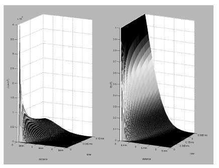
In the previous chapter we considered the special case of Maxwell’s equations with time-harmonic sources. If the field sources have arbitrary time dependence, then we must work with the time-dependent curl and divergence equations 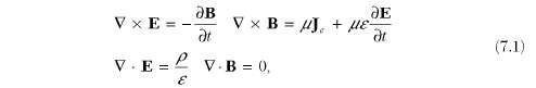 where Je = σE + Jsource and (μ, ε) = ( μr μ0 ,εr ε0 ). Current Sheet Above a Conducting Half-Space The simplest example of transient current induction is that produced by a magnetic field tangential to a conducting half-space that is switched on at t = 0. This field can be thought of as being produced by an infinite sheet with a uniform surface current density that is parallel to the conducting half-space. Neglecting the displacement current we have  inside the metal and taking the curl of this equation and using 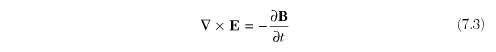 we obtain  For an external field B(t) = B0θ(t)j, the differential equation with initial conditions becomes  where θ(t) is zero for t < 0 and 1 for t ≥ 0. Taking the Laplace transform of both the differential equation and initial conditions gives 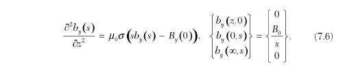 where By(0) = 0. The solution to this equation is  Applying the boundary conditions we have A = 0 and  Performing the inverse Laplace transform in MATLAB 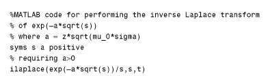 gives the field in the time-domain 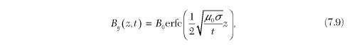 where the complementary error function is given by 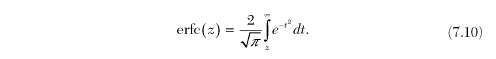 The eddy current is given by μ0Jx= -∂By/∂z so that using the identity 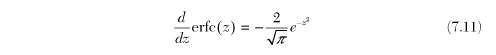 finally gives the eddy current 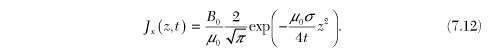 Equation 7.5 may be solved numerically using an explicit finite difference numerical method 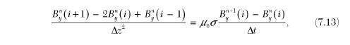 where the spatial and time derivatives are evaluated using central difference and forward difference schemes, respectively. The magnetic field is then advanced in time at each grid point according to 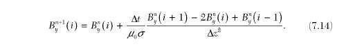 This explicit method is stable for Δt ≤ μ0σΔz2/2. Once the field is known, the current density may be calculated according to  Implicit methods, such as the Crank-Nicholson method, may also be used for greater stability and accuracy. The following MATLAB program calculates the penetration of magnetic fields and the induced currents inside the metal: 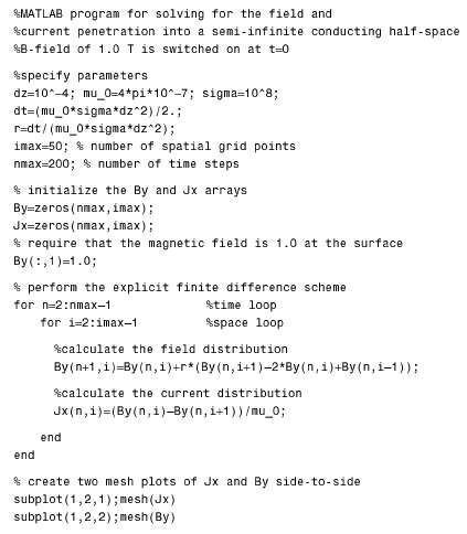 The output of this program is shown in Figure 7.1. Axis labels and the figure perspectives were adjusted in the window show.
|
 giving