Preface
The first generation of fiber-optic communication systems debuting in 1980 operated at a meager bit rate of 45 Mb/s and required signal regeneration every 10 km or so. However, by 1990 further advances in lightwave technology not only increased the bit rate to 10 Gb/s (by a factor of 200) but also allowed signal regeneration after 80 km or more. The pace of innovation in all fields of lightwave technology only quickened during the 1990s, as evident from the development and commercialization of erbium-doped fiber amplifiers, fiber Bragg gratings, and wavelength-division-multiplexed lightwave systems. By 2001, the capacity of commercial terrestrial systems exceeded 1.6 Tb/s. At the same time, the capacity of transoceanic lightwave systems installed worldwide exploded. A single transpacific system could transmit information at a bit rate of more than 1 Tb/s over a distance of 10,000 km without any signal regeneration. Such a tremendous improvement was possible only because of multiple advances in all areas of lightwave technology. Although commercial development slowed down during the economic downturn that began in 2001, it was showing some signs of recovery by the end of 2004, and lightwave technology itself has continued to grow. The primary objective of this two-volume book is to provide a comprehensive and up-to-date account of all major aspects of lightwave technology. The first volume, subtitled Components and Devices, is devoted to a multitude of silica- and semiconductor-based optical devices. The second volume, subtitled Telecommunication Systems, deals with the design of modern lightwave systems; the acronym LT1 is used to refer to the material in the first volume. The first two introductory chapters cover topics such as modulation formats and multiplexing techniques employed to form an optical bit stream. Chapters 3 through 5 consider the degradation of such an optical signal through loss, dispersion, and nonlinear effects during its transmission through optical fibers and how they affect the system performance. Chapters 6 through 8 focus on the management of the degradation caused by noise, dispersion, and fiber nonlinearity. Chapters 9 and 10 cover the engineering issues related to the design of WDM systems and optical networks. This text is intended to serve both as a textbook and a reference monograph. For this reason, the emphasis is on physical understanding, but engineering aspects are also discussed throughout the text. Each chapter also includes selected problems that can be assigned to students. The book's primary readership is likely to be graduate students, research scientists, and professional engineers working in fields related to lightwave technology. An attempt is made to include as much recent material as possible so that students are exposed to the recent advances in this exciting field. The reference section at the end of each chapter is more extensive than what is common for a typical textbook. The listing of recent research papers should be helpful to researchers using this book as a reference. At the same time, students can benefit from this feature if they are assigned problems requiring reading of the original research papers. This book may be useful in an upper-level graduate course devoted to optical communications. It can also be used in a two-semester course on optoelectronics or lightwave technology. A large number of persons have contributed to this book either directly or indirectly. It is impossible to mention all of them by name. I thank my graduate students and the students who took my course on optical communication systems and helped improve my class notes through their questions and comments. I am grateful to my colleagues at the Institute of Optics for numerous discussions and for providing a cordial and productive atmosphere. I thank, in particular, Renè Essiambre and Qiang Lin for reading several chapters and providing constructive feedback. Last, but not least, I thank my wife Anne and my daughters, Sipra, Caroline, and Claire, for their patience and encouragement. Govind P. Agrawal Rochester, NY |
Chapter 9.4.1 - Amplitude Fluctuations
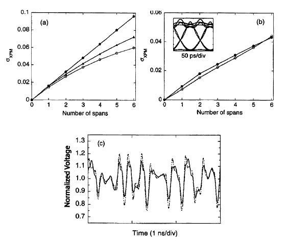
9.4.1 Amplitude FluctuationsConsider the source of amplitude fluctuations first. As discussed in Section 4.2, XPM originates from the nonlinear nature of the refractive index, which produces a phase shift that depends on the bit patterns of neighboring channels. Strictly speaking, the XPM-induced phase shift should not affect system performance if the GVD effects were negligible. However, any dispersion in fiber converts pattern-dependent phase shifts to power fluctuations, reducing the SNR at the receiver. This conversion can be understood by noting that time-dependent phase changes lead to frequency chirping that affects dispersion-induced broadening of the signal. Such XPM-induced power fluctuations can become quite large for large values of dispersion parameter and channel powers. In a dispersion-managed system, they also depend on the dispersion map employed. The pump-probe analysis developed in Sections 4.2.3 is often used to estimate the level of XPM-induced power fluctuations on a CW probe as it travels down the fiber link with a data channel acting as a pump at a different wavelength [70]-[73]. Figure 9.13(a) shows fluctuation level σXPM of a probe channel as a function of link length when it propagates with a 10-Gb/s channel separated by 50 GHz and launched with 10-mW power [80]. Each span consists of 60 km of standard fiber, followed with 12 km of DCF, resulting in zero dispersion on average. Symbols are used to compare the pump-probe approach (filled circles) with the numerical solutions obtained by solving the NLS equation (open circles). Clearly, the pump-probe approach provides an order-of-magnitude estimate as it ignores nonlinear distortion of the pump channel. The curve with triangles is obtained when pump distortions are taken into account. The level of pump distortion can be reduced if the DCF length is shortened to 10.8 km so that the average dispersion of the link is anomalous, and soliton effects become important. As seen in Figure 9.13(b), the pump-probe approach is then in better agreement with full numerical simulations. The inset shows the eye diagram for the pump channel after 6 spans. Temporal variations of the probe power (normalized to 1 at the input end) after five spans are displayed in part (c). Solid and dashed curves compare the solution of the NLS equation with the improved pump-probe approach. The important point is that the XPM generates power fluctuations that become larger than 20% after only 300 km. As a result, the SNR at the receiver end will be reduced considerably for all channels. Clearly, one must design a WDM system to minimize them.
Figure 9.13: Standard deviation of XPM-induced probe fluctuations as a function of link length (each span is 60 km) when the DCF length in each span is (a) 12 km or (b) 10.8 km. (c) Probe fluctuations after 5 spans with an input level normalized to 1. (After Ref. [80]; ©2000 IEEE.)
Figure 9.14: Measured standard deviation of probe fluctuations as a function of channel spacing with (circles) and without (squares) dispersion compensation. Triangles represent the data obtained under field conditions. Inset shows a temporal trace of probe fluctuations for Δλ, = 0.4 nm. (After Ref. [78]; ©2000 IEEE.)
where σXPM is the value calculated with the pump-probe method [80]. The basic assumption is that XPM-induced amplitude fluctuations enhance the noise level of 1 bits (but leave the 0 bits relatively unaffected), and this noise can be added to other noise sources, assuming that it is governed by an independent Gaussian process. Such an approach works reasonably well when the WDM signal is in the the NRZ format. In the case of RZ format, one must include the impact of XPM-induced timing jitter, a topic we turn to next. |