Preface
The first generation of fiber-optic communication systems debuting in 1980 operated at a meager bit rate of 45 Mb/s and required signal regeneration every 10 km or so. However, by 1990 further advances in lightwave technology not only increased the bit rate to 10 Gb/s (by a factor of 200) but also allowed signal regeneration after 80 km or more. The pace of innovation in all fields of lightwave technology only quickened during the 1990s, as evident from the development and commercialization of erbium-doped fiber amplifiers, fiber Bragg gratings, and wavelength-division-multiplexed lightwave systems. By 2001, the capacity of commercial terrestrial systems exceeded 1.6 Tb/s. At the same time, the capacity of transoceanic lightwave systems installed worldwide exploded. A single transpacific system could transmit information at a bit rate of more than 1 Tb/s over a distance of 10,000 km without any signal regeneration. Such a tremendous improvement was possible only because of multiple advances in all areas of lightwave technology. Although commercial development slowed down during the economic downturn that began in 2001, it was showing some signs of recovery by the end of 2004, and lightwave technology itself has continued to grow. The primary objective of this two-volume book is to provide a comprehensive and up-to-date account of all major aspects of lightwave technology. The first volume, subtitled Components and Devices, is devoted to a multitude of silica- and semiconductor-based optical devices. The second volume, subtitled Telecommunication Systems, deals with the design of modern lightwave systems; the acronym LT1 is used to refer to the material in the first volume. The first two introductory chapters cover topics such as modulation formats and multiplexing techniques employed to form an optical bit stream. Chapters 3 through 5 consider the degradation of such an optical signal through loss, dispersion, and nonlinear effects during its transmission through optical fibers and how they affect the system performance. Chapters 6 through 8 focus on the management of the degradation caused by noise, dispersion, and fiber nonlinearity. Chapters 9 and 10 cover the engineering issues related to the design of WDM systems and optical networks. This text is intended to serve both as a textbook and a reference monograph. For this reason, the emphasis is on physical understanding, but engineering aspects are also discussed throughout the text. Each chapter also includes selected problems that can be assigned to students. The book's primary readership is likely to be graduate students, research scientists, and professional engineers working in fields related to lightwave technology. An attempt is made to include as much recent material as possible so that students are exposed to the recent advances in this exciting field. The reference section at the end of each chapter is more extensive than what is common for a typical textbook. The listing of recent research papers should be helpful to researchers using this book as a reference. At the same time, students can benefit from this feature if they are assigned problems requiring reading of the original research papers. This book may be useful in an upper-level graduate course devoted to optical communications. It can also be used in a two-semester course on optoelectronics or lightwave technology. A large number of persons have contributed to this book either directly or indirectly. It is impossible to mention all of them by name. I thank my graduate students and the students who took my course on optical communication systems and helped improve my class notes through their questions and comments. I am grateful to my colleagues at the Institute of Optics for numerous discussions and for providing a cordial and productive atmosphere. I thank, in particular, Renè Essiambre and Qiang Lin for reading several chapters and providing constructive feedback. Last, but not least, I thank my wife Anne and my daughters, Sipra, Caroline, and Claire, for their patience and encouragement. Govind P. Agrawal Rochester, NY |
 TABLE OF CONTENTS
 Chapter 9.5.3 - Polarization Interleaving of Channels
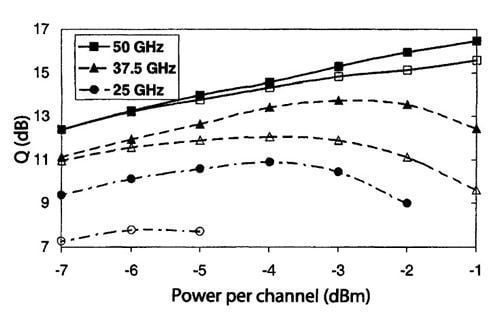
9.5.3 Polarization Interleaving of ChannelsAs discussed in Section 8.5.3, the impact of intrachannel nonlinear effects can be reduced considerably by ensuring that the neighboring bits in a channel are orthogonally polarized. The same idea can be extended to the case of interchannel nonlinearities by designing WDM systems such that the bit streams in two neighboring channels are orthogonally polarized [120]—[123]. Such a scheme is relatively easy to implement in practice. Figure 9.20 shows the experimental setup used typically for this purpose. The even and odd number channels are multiplexed together into two separate branches, whose states of polarization (SOPs) are adjusted using polarization controllers such that they are orthogonal. A polarization beam combiner or a device known as the channel polarization interleaver is then used to create a WDM signals whose neighboring channels are orthogonally polarized. Why should polarization interleaving help in reducing the impact of interchannel nonlinear effects? The reason is that both XPM and FWM depend on the SOPs of the interacting channels. When two pulses in neighboring channels collide and interact through XPM, the phase, frequency, and temporal shifts induced by such a collision depend on the relative SOPs of the two channels. More precisely, the factor of 2 appearing in the last term in Eqs. (9.4.3) and (9.4.4) is replaced with 2/3, when the channels are orthogonally polarized [39]. As a result, interchannel collisions should produce smaller phase shifts and lead to much less amplitude and timing jitters. Before reaching this conclusion, however, one should address the impact of polarization-mode dispersion (PMD) on channel polarizations [124]-[127]. As discussed in Section 3.4, PMD results from fluctuating residual birefringence inherent in all fibers used for designing lightwave systems. Its main effect is to change the SOP of each channel in a random fashion. If the two channels change their SOPs in a random fashion but remain nearly orthogonal, the technique of polarization interleaving can still be beneficial. In the language of Section 3.4, the Stokes vector of each channel would move in a random fashion on the Poincare sphere but the Stokes vectors associated with two neighboring channels would remain antiparallel to each other. The important question is over what lengths neighboring channels can maintain orthogonal SOPs in spite of birefringence fluctuations. As discussed in Section 3.4, the frequency dependence of the Stokes vector is governed by Eq. (3.4.27) and depends on the PMD vector. The length over which the relative SOP of neighboring channels can change significantly is known as the diffusion length Ldiff. It depends on the PMD parameter of the fiber Dpand the channel spacing Ωch through the relation Ldiff = (DpΩch)-2. This length can vary over a wide range (<100 to >5,000 km) depending on the values of Dpand Ωch. For two channels spaced 50 GHz apart Ldiff is about 1,000 km, if we use Dp = 0.1 ps/km1/2 as a typical value for the PMD parameter. This estimate suggests that the polarization-interleaving technique is appropriate for suppressing interchannel nonlinear effects in WDM systems when fibers with relatively low values of Dpare employed and channel spacing is less than 100 GHz. Figure 9.23 shows the results of numerical simulations for a 9,000-km dispersion-managed WDM system [122]. The 45-km-long dispersion map employs 28.5-km and 16.5-km sections with dispersions of 20 and -40 ps/(km-nm), respectively, and its residual dispersion is compensated every 500 km. Each 10-Gb/s channel carries an RZ bit stream with 33% duty cycle at an effective bit rate of 12.3 Gb/s because of FEC coding. Channel spacing is varied in the range of 25 to 50 GHz, and the PMD parameter of the fiber has a value of Dp = 0.06 ps/km1/2. The Q factors were calculated numerically for several input power levels when neighboring channels were either copolarized or orthogonally polarized. A comparison of Q factors in the two cases, plotted as a function of launched power/channel for three channel spacings in Figure 9.23, shows that the use of polarization interleaving can improve the Q factor by more than 2 dB for a 25-GHz channel spacing but this advantage almost disappears when channel spacing is 50 GHz. The experiments performed over a distance of 6,500 km with 25-GHz channel spacing showed an improvement of more than 1 dB with the use of polarization interleaving [122].
Figure 9.23: Q factors after 9,000 km as a function of launched power for three values of channel spacings when neighboring channels are copolarized (empty symbols) or orthogonally polarized (rilled symbols) for a PMD parameter Dp= 0.06 ps/km1/2. (After Ref. [122]; ©2002 IEEE.)
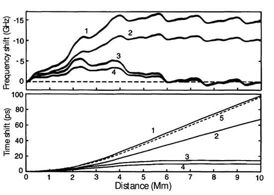
Figure 9.24: Collision-induced frequency and temporal shifts for a pulse in a channel surrounded by four channels with 75-GHz spacing on each side. Curves 1 and 2 represent the cases of copolarized and orthogonally polarized channels, respectively. Curves 3 and 4 show the improvement realized with sliding-frequency filters. The dashed line shows the prediction of an analytical model. (After Ref. [93]); ©1999 OSA.) |