Preface
The first generation of fiber-optic communication systems debuting in 1980 operated at a meager bit rate of 45 Mb/s and required signal regeneration every 10 km or so. However, by 1990 further advances in lightwave technology not only increased the bit rate to 10 Gb/s (by a factor of 200) but also allowed signal regeneration after 80 km or more. The pace of innovation in all fields of lightwave technology only quickened during the 1990s, as evident from the development and commercialization of erbium-doped fiber amplifiers, fiber Bragg gratings, and wavelength-division-multiplexed lightwave systems. By 2001, the capacity of commercial terrestrial systems exceeded 1.6 Tb/s. At the same time, the capacity of transoceanic lightwave systems installed worldwide exploded. A single transpacific system could transmit information at a bit rate of more than 1 Tb/s over a distance of 10,000 km without any signal regeneration. Such a tremendous improvement was possible only because of multiple advances in all areas of lightwave technology. Although commercial development slowed down during the economic downturn that began in 2001, it was showing some signs of recovery by the end of 2004, and lightwave technology itself has continued to grow. The primary objective of this two-volume book is to provide a comprehensive and up-to-date account of all major aspects of lightwave technology. The first volume, subtitled Components and Devices, is devoted to a multitude of silica- and semiconductor-based optical devices. The second volume, subtitled Telecommunication Systems, deals with the design of modern lightwave systems; the acronym LT1 is used to refer to the material in the first volume. The first two introductory chapters cover topics such as modulation formats and multiplexing techniques employed to form an optical bit stream. Chapters 3 through 5 consider the degradation of such an optical signal through loss, dispersion, and nonlinear effects during its transmission through optical fibers and how they affect the system performance. Chapters 6 through 8 focus on the management of the degradation caused by noise, dispersion, and fiber nonlinearity. Chapters 9 and 10 cover the engineering issues related to the design of WDM systems and optical networks. This text is intended to serve both as a textbook and a reference monograph. For this reason, the emphasis is on physical understanding, but engineering aspects are also discussed throughout the text. Each chapter also includes selected problems that can be assigned to students. The book's primary readership is likely to be graduate students, research scientists, and professional engineers working in fields related to lightwave technology. An attempt is made to include as much recent material as possible so that students are exposed to the recent advances in this exciting field. The reference section at the end of each chapter is more extensive than what is common for a typical textbook. The listing of recent research papers should be helpful to researchers using this book as a reference. At the same time, students can benefit from this feature if they are assigned problems requiring reading of the original research papers. This book may be useful in an upper-level graduate course devoted to optical communications. It can also be used in a two-semester course on optoelectronics or lightwave technology. A large number of persons have contributed to this book either directly or indirectly. It is impossible to mention all of them by name. I thank my graduate students and the students who took my course on optical communication systems and helped improve my class notes through their questions and comments. I am grateful to my colleagues at the Institute of Optics for numerous discussions and for providing a cordial and productive atmosphere. I thank, in particular, Renè Essiambre and Qiang Lin for reading several chapters and providing constructive feedback. Last, but not least, I thank my wife Anne and my daughters, Sipra, Caroline, and Claire, for their patience and encouragement. Govind P. Agrawal Rochester, NY |
Chapter 9.6.2 - Dispersion Fluctuations
9.6.2 Dispersion FluctuationsSo far we have treated the dispersion of all fiber sections used to form a dispersion-managed fiber link as being uniform along the section length. We have also assumed that dispersion does not change with time. Both these assumptions are questionable for realistic fibers. The zero-dispersion wavelength λ0 of a fiber depends on its core diameter, which can vary along the fiber length by a small amount (a few percent) in a random fashion during the fiber-pulling stage. Any variations in λ0 manifest as changes in the value of the dispersion parameter D(λ) at the channel wavelength. Although such dispersion variations are static in nature, they can affect system performance whenever nonlinear effects are not negligible along the link. For this reason, dispersion fluctuations have attracted the most attention in the context of solitons [151]-[153]. A second source of dispersion fluctuations is related to environmental changes. If the temperature of the fiber changes at a given location, the local dispersion would also change with it because D also depends on temperature [154]-[156]. Such dynamic fluctuations are of considerable concern for 40-Gb/s channels for which dispersion tolerance is relatively tight. In a simple model, D is assumed to vary with λ as
where S0 is the dispersion slope at the zero-dispersion wavelength λ0. Both S0 and λ0 vary along the fiber length and with temperature. Such variations affect system performance because the BER or the Q factor is sensitive to the distribution of dispersion along the link length. In the case of a linear system, their impact can be completely eliminated by employing a dynamic dispersion-compensation scheme (see Section 7.7.1). However, such a scheme does not work perfectly when nonlinear effects play a significant role. To study the impact of dispersion fluctuations on the performance of a WDM channel operating at 40 Gb/s, the NLS equation is solved numerically, while including both the amplitude and phase fluctuations induced by the noise added by amplifiers. Dispersion fluctuations are included by writing the local dispersion parameter as
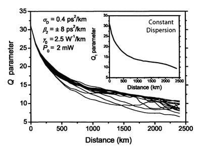
where Figure 9.31 shows how Q changes with distance for 15 different realizations of the random variable δβ characterized by a standard deviation of σD= 0.4 ps2/km [153]. In these simulations, the dispersion map consisted of two fiber sections of nearly equal lengths (5 km) with
Figure 9.31: Q factor as a function of distance for 15 realizations of dispersion fluctuations for a 40-Gb/s channel. The inset shows Q values expected in the absence of dispersion fluctuations. The input peak power of 6-ps pulses was 2 mW. (After Ref. [153]; ©2003 IEEE.)
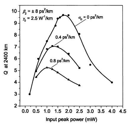
Figure 9.32: Worst-case Q factor for a 40-Gb/s channel at a distance of 2,400 km as a function of input peak power for three values of σD. (After Ref. [153]; ©2003 IEEE.) |