9.4.2 Timing Jitter

XPM interaction among neighboring channels can induce considerable timing jitter. The situation is somewhat different from the intrachannel case discussed in Section 8.4.2 where all pulses travel with the same speed and thus remain overlapped throughout the fiber. In contrast, pulses belonging to different channels travel at different speeds in a WDM system and walk through each other at a rate that depends on the wavelength difference of the two channels involved. Since XPM can occur only when pulses overlap in the time domain, one must include the walk-off effects in any study of interchannel XPM [86]-[96].

Physically, timing jitter is a consequence of the frequency shifts experienced by pulses in one channel as they overlap with pulses in other neighboring channels. Temporal overlapping of optical pulses in two neighboring channels is referred to as a collision. As a faster-moving pulse belonging to one channel collides with and passes through a pulse in another channel, the XPM-induced chirp shifts the pulse spectrum first toward the red side and then toward the blue side. In a lossless fiber, most collisions are perfectly symmetric, resulting in no net spectral shift, and hence no temporal shift, at the end of the collision.

In a loss-managed system with optical amplifiers placed periodically along the link, power variations make collisions between pulses of different channels asymmetric, resulting in a net frequency shift, and hence in a net temporal shift, that depends on the magnitude of channel spacing. Physically speaking, the speed of pulses belonging to a WDM channel depends on its carrier frequency, and any change in this frequency slows down or speeds up their speed, depending on the direction in which frequency changes. A constant temporal shift would be of little consequence if it were the same for all pulses. However, the XPM-induced shift in the pulse position is different for different pulses because it depends on the bit patterns and wavelengths of other channels, and thus manifests as a timing jitter at the receiver end. This timing jitter degrades the eye pattern, especially for closely spaced channels, and leads to an XPM-induced power penalty that depends on channel spacing and the type of fibers used for the WDM link. The power penalty increases for fibers with large GVD and for WDM systems designed with a small channel spacing and can become quite large when channel spacing is reduced to below 100 GHz. Such a restriction on channel spacing translates into a low spectral efficiency.

Mathematically, the effects of interchannel collisions on the performance of WDM systems can be best understood by considering the simplest case of two WDM channels separated by Ω_ch. Using the NLS equation (8.1.2) with

and neglecting the FWM terms, pulses in each channel are found to evolve according to the following two coupled equations:

where δ = β₂Ω_ch measure of the mismatch between the group velocities of the two channels. In writing these equations, the common carrier frequency is chosen to be in the center of the two channels.

It is useful to define the collision length L_coll as the distance over which pulses in different channels remain overlapping during a collision before separating. It is difficult to determine precisely the instant at which a collision begins or ends. One convention uses 2T_sfor the duration of the collision, where T_sis the full width at the half-maximum (FWHM) of each pulse, assuming that a collision begins and ends when two pulses overlap at their half-power points [86]. In another, the duration T_bof bit slot is used for this purpose. In the case of RZ format, the two conventions are related to each other because T_s - T_b/2 for a 50% duty cycle. Since 5 is a measure of the relative speed of two pulses, the collision length can be written as

where B is the bit rate and Δv_ch is the channel spacing. As an example, if we use B = 10 Gb/s and β₂ = 5 ps²/km, L_coll ≈ 32 km for a channel spacing of 100 GHz and it reduces to below 8 km for a 40-Gb/s system. Even smaller values can occur if standard fibers are used with β₂ ≈ 20 ps²/km. In contrast, L_coll can exceed 100 km when low-dispersion fibers are employed with a small channel spacing.

The last term in Eqs. (9.4.3) and (9.4.4) is due to XPM-induced coupling between two channels and is responsible for the temporal and frequency shifts during a collision. Similar to the analysis used in Section 8.4.2 for intrachannel XPM, we can employ the variational or the moment method to calculate these shifts [95]. In fact, details are similar to the intrachannel case, and the moment equations for the pulse parameters are almost identical to Eqs. (8.4.11) through (8.4.14). The only difference is that one needs to take into account the group-velocity mismatch between the two pulses. If we assume that pulses in two channel are identical in all respects, these equations take the form (after dropping the subscript on T and C)

where µ = Δt/T. Notice that the temporal shift depends on the net frequency separation Ω_ch + ΔΩ between the two channels, where Ω_ch is the constant channel spacing and ΔΩis the XPM-induced frequency shift. Similarly, Δt represents net temporal spacing between two pulses and consists of two parts Δt_pand Δt_XPM. The first part represents the collision of two pulses because of a finite value of Ω_ch, while the second part is due to XPM-induced coupling between them.

The net XPM-induced frequency shift ΔΩ can be calculated by integrating Eq. (9.4.8) over a distance longer than the collision length such that pulses are well separated before and after the collision. Using z = z_c + µT/δ where z_cis the location where pulses overlap completely (center of collision), the result can be written as

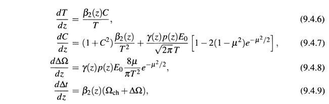
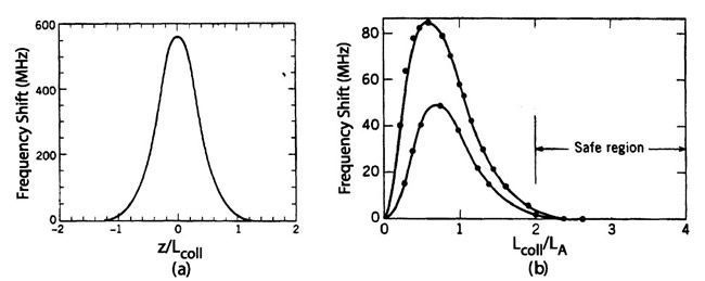
where we assumed that pulse width does not change significantly during a collision. The parameter µ ≈ Δt_p / 2T changes from negative to positive, becoming zero in the center of the collision where pulses overlap fully. Since the integrand is an odd function of µ when γ and p are z-independent, the integral in Eq. (9.4.10) vanishes in this case. This can happen if (1) a collision is complete entirely within one fiber section with constant γ and (2) distributed amplification is used such that p ≈ 1. Under such conditions, two colliding pulses do not experience any temporal shift within their assigned bit slots.

Figure 9.15(a) shows how the frequency of the slow-moving pulse changes during the collision of two 50-ps solitons when channel spacing is 75 GHz. The frequency shifts up first as two pulses approach each other, reaches a peak value of about 0.6 GHz at the point of maximum overlap, and then decreases back to zero as two pulses separate. The maximum frequency shift depends on the channel spacing. It can be calculated by replacing the upper limit in Eq. (9.4.10) with 0. When p = 1 and γ is constant during a collision, it is given by

where L_NL = (γP₀) ^-1 is the nonlinear length and Δv_ch is the channel spacing. One can follow the same procedure for the collision of two solitons with an amplitude of the form sech(t/T₀) to find Δf_max = (3π²T²₀Δv_ch)^-1. For 40-Gb/s channels spaced 100 GHz apart, this maximum frequency shift can exceed 10 GHz.

Most interchannel collisions are rarely symmetric in WDM systems for a variety of reasons. When fiber losses are compensated periodically through lumped amplifiers, p(z) is never an even function with respect to the center of collision. Physically, large peak-power variations occurring over a collision length destroy the symmetric nature of the collision. As a result, pulses suffer net frequency and temporal shifts after the collision is over. Equation (9.4.9) can be used to calculate the residual frequency shift for a given functional form of p(z). Figure 9.15(b) shows the residual shift as a function of the ratio L_coll/L_A where L_A is the amplifier spacing, in the case of solitons [86]. The residual frequency shift increases rapidly as L_coll approaches L_Aand becomes ~0.1 GHz. Such shifts are not acceptable in practice since they accumulate over multiple collisions and produce velocity changes large enough to move the pulse out of its assigned bit slot. When L_coll is so large that a collision lasts over several amplifier spacings, the effects of gain-loss variations begin to average out, and the residual frequency shift decreases. As seen in Figure 9.15(b), it virtually vanishes for L_coll > 2L_A(safe region).

Figure 9.15: (a) Frequency shift during collision of two 50-ps solitons with 75-GHz channel spacing, (b) Residual frequency shift after a collision because of lumped amplifiers (L_A = 20 and 40 km for lower and upper curves, respectively). Numerical results are shown by solid dots. (After Ref. [86]; ©1991 IEEE.)

The preceding two-channel analysis focuses on a single collision of two pulses. Several other issues must be considered when calculating the timing jitter. First, neighboring pulses in a given channel experience different number of collisions. This difference arises because adjacent pulses in a given channel interact with two different bit groups, shifted by one bit period. Since 1 and 0 bits occur in a random fashion, different pulses of the same channel are shifted by different amounts. Second, collisions involving more than two pulses can occur and should be considered. Third, a residual frequency shift always occurs when pulses in two different channels overlap at the input of the transmission link because their collisions are always incomplete (since the first half of the collision is absent). Such residual frequency shifts are generated only over the first few amplification stages but pertain over the whole transmission length and become an important source of timing jitter [87].

An entirely different situation is encountered in dispersion-managed systems where a collision may not be complete before the dispersion changes suddenly its nature at the end of a fiber section. As soon as the colliding pulses enter the fiber section with opposite dispersion characteristics, the pulse traveling faster begins to travel slower, and vice versa. Moreover, because of high values of local dispersion, the speed difference between two channels is relatively large. Also, the pulse width changes in each map period and can become quite large in some regions. The net result is that two colliding pulses move in a zigzag fashion and pass through each other many times before they separate from each other because of the much slower relative motion governed by the average value of GVD. Since the effective collision length becomes much larger than the map period (and the amplifier spacing), the condition L_coll > 2L_Ais satisfied even when soliton wavelengths differ by 20 nm or more. This feature makes it possible to design WDM systems with a large number of channels.

The residual frequency shifts encountered in dispersion-managed systems depend on a large number of parameters, including map period, map strength, and amplifier spacing [90]-[96]. As before, residual frequency shifts occurring during complete collisions average out to zero. However, not all collisions are complete. For example, if pulses overlap initially, the incomplete nature of the collision will produce some residual frequency shift. The zigzag motion of pulses can also produce frequency shifts if two pulses approach each other near the junction of opposite-dispersion fibers because they will reverse direction before crossing each other. Such partial collisions can result in large frequency shifts and thus produce a relatively large timing jitter. This situation can be avoided by optimizing the dispersion map used for a WDM system appropriately [95].

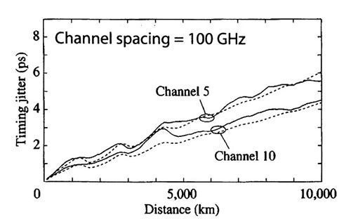
Figure 9.16: Growth of timing jitter in two channels as a function of distance for a 10-channel WDM system designed with a 100-km periodic dispersion map. Numerical (solid curves) and semianalytic (dashed curves) results are compared for 10-Gb/s channels spaced apart by 100 GHz. (After Ref. [96]; ©2000 IEEE.)

An accurate estimate of XPM-induced timing jitter for a WDM system requires numerical solutions of the NLS equation that become quite time-consuming as the number of channels increases. A semianalytic approach based on the moment method has been used with success [96]. It uses the optical field found numerically for a single pulse in each isolated channel (a relatively fast calculation) to calculate the timing jitter in all WDM channels by performing the average over random bit patterns in an analytic fashion. Figure 9.16 compares the results obtained using such an approach (dashed line) with those calculated using full numerical simulations (solid line) for a 10-channel dispersion-managed WDM system. All channels operate at 10 Gb/s and are spaced apart by 100 GHz. The dispersion map consists of a 95.6-km fiber with D = 4 ps/(km-nm) followed with 4.4 km of DCF with D = -85 ps/(km-nm). An amplifier is located in the middle of each fiber span. The peak power of each pulse representing 1 bit is taken to be 3.13 mW.

A noteworthy feature of Figure 9.16 is that timing jitter does not increase monoton-ically and exhibits periodic humps. The hump period is related to the distance over which pulses in two neighboring channels separate fully, after following a zigzag path, and is given by L_h= T_b / (₂ΔΩ_ch), where T_b is the duration of each bit slot and ₂ is the average value of β₂. For the parameter values used for Figure 9.16, L_h is about 1,600 km. The other important feature of Figure 9.16 is that timing jitter is larger for the central channel compared with the first or last channel. This is easily understood by noting that pulses in the central channel collide with pulses in channels located on both sides and thus experience more jitter.