Digital Techniques for Wideband Receivers, Second Edition

14.6: BACKWARD PREDICTION AND MODIFIED COVARIANCE METHOD [3, 4, 13, 19, 22]

14.6 BACKWARD PREDICTION AND MODIFIED COVARIANCE METHOD [3, 4, 13, 19, 22]

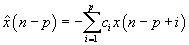
The two methods discussed in the next section can be considered as subcategories of the AR method. The purpose of introducing the backward prediction and modified covariance method is to prepare for the discussion of the Burg method, because this concept is used in the Burg method. The linear prediction discussed in previous sections is referred to as the forward prediction, since past data are used to predict the present data. In the backward prediction, the past data are predicted from the previous data. This may sound a little absurd, because the previous data are already known. However, if one considers the time series as a data set rather than a sequence occurring in time, one can linearly predict in either direction. The backward prediction can be written as

(14.36)

where c i is the backward prediction coefficient.

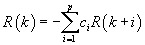
The relation between the backward and forward coefficients can be found as follows. The Yule-Walker equation can be obtained from the above equation by multiplying both sides by x* ( n - p - k) and taking the expectation value. The result is

(14.37)

From the definition of autocorrelation, this equation can be written as

(14.38)

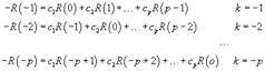
Written in separate equations, the result is

(14.39)

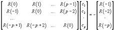
In matrix form, it is

(14.40)

Now, let us find the relation between the forward prediction coefficients a i and the backward prediction coefficients c i. Taking the complex...

UNLIMITED FREE
ACCESS
TO THE WORLD'S BEST IDEAS

SUBMIT
Already a GlobalSpec user? Log in.

This is embarrasing...

An error occurred while processing the form. Please try again in a few minutes.

Customize Your GlobalSpec Experience

Category: Digital Counters
Finish!
Privacy Policy

This is embarrasing...

An error occurred while processing the form. Please try again in a few minutes.