4.1 Position of the problem

We are examining two discrete time processes:

• of the 2 ^nd order;

• not necessarily wide sense stationary (WSS) (thus they do not necessarily have a spectral density).

is called the state process and is the process (physical for example) that we are seeking to estimate, but it is not accessible directly.

is called the observation process, which is the process we observe (we observe a trajectory which allows us to estimate the corresponding trajectory ).

A traditional example is the following:

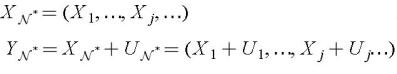
where is also a random process.

We thus say that the state of the process is perturbed by a parasite noise . (perturbation due to its measurement, transmission, etc.).

In what follows, the hypothesis and data will be admitted:

• X _j and Y _j ? L ² ( dP);

• , we know EX _j, cov ( X _i, Y _j), cov ( Y _i, Y _j).

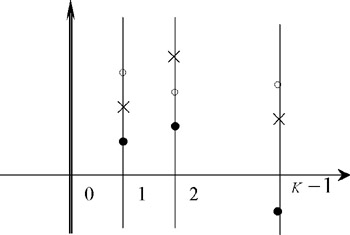
PROBLEM. Having observed (or registered) a trajectory of up to the instant K ? 1, we want, for a given instant p, to determine the value " which best approaches x _p (unknown)".

Figure 4.1: Three trajectories

and which is unknown

If:

• p < K ? 1 we speak of smoothing;

• p = k ? 1 we speak of filtering;

• p > K ? 1 we speak of prediction.