Practical Energy Efficiency Optimization

Presenting basic information for optimizing power plants, this book uses review exercises and practical case studies to provide real-world applications on maintaining optimal efficiency.
Consider the case of a process heater whose efficiency varies with load percentage as shown in the previous example. The same heater will perform differently with the passage of time (1 year, 1 1/2 years, 2 years, etc.). Although the efficiency pattern may remain the same in all these load conditions, the observed efficiency for the same load will be somewhat lower as time passes. Hence, necessary run length will have to be incorporated as a factor in the model. A typical case is shown following and in figure 2-5.
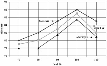
Table 2-5 shows the behavioral pattern of the heater with passage of time called onstream hours. It is possible to predict the behavioral pattern after a certain time interval, for taking corrective action. For this purpose, a two-variable model is built for the heater with load and operating hours as two independent variables. This is a very important method for heat exchangers/coolers/condensers, as they develop fouling with time and even after de-scaling, the original heat transfer rate is seldom achieved. This data when converted into a model gives
| Load % | Base case | After 1 year | After 2 years |
|---|---|---|---|
| 70 | 80 | 79 | 78.0 |
| 80 | 82 | 80 | 78.0 |
| 90 | 85 | 83 | 81.5 |
| 100 | 88 | 87 | 85.5 |
| 110 | 85 | 82 | 81.0 |
| (2.11) | |
where op. mo. is the operating month.
This model may be used to predict the efficiency at any load over a reasonable operating month. For...