 | Although DSP has long been considered an EE topic, recent developments have also generated signifi cant interest from the computer science community. DSP applications in the consumer market, such as bioinformatics, the MP3 audio format, and MPEG-based cable/satellite television have fueled a desire to understand this technology outside of hardware circles. Designed for upper division engineering and computer science students as well as practicing engineers, Digital Signal Processing Using MATLAB and Wavelets emphasizes the practical applications of signal processing. Over 100 MATLAB examples and wavelet techniques provide the latest applications of DSP, including image processing, games, fi lters, transforms, networking, parallel processing, and sound. The book also provides the mathematical processes and techniques needed to ensure an understanding of DSP theory. Designed to be incremental in diffi culty, the book will benefi t readers who are unfamiliar with complex mathematical topics or those limited in programming experience. Beginning with an introduction to MATLAB programming, it moves through filters, sinusoids, sampling, the Fourier transform, the z-transform and other key topics. An entire chapter is dedicated to the discussion of wavelets and their applications. A CD-ROM (platform independent) accompanies the book and contains source code, projects for each chapter, and the fi gures contained in the book. FEATURES:
|
![$y[n] = 2 x[n-3]$](/RefArticleImages/AC20BF92F42FAE8F4B1DC1261E2AD45F_img142_9.gif) . If the
down-samplers and up-samplers are included, then the 2 term drops out.
This is shown later. First, we will start, as usual,
with Figure 9.12, an updated filter bank for
four coefficients in each filter.
. If the
down-samplers and up-samplers are included, then the 2 term drops out.
This is shown later. First, we will start, as usual,
with Figure 9.12, an updated filter bank for
four coefficients in each filter.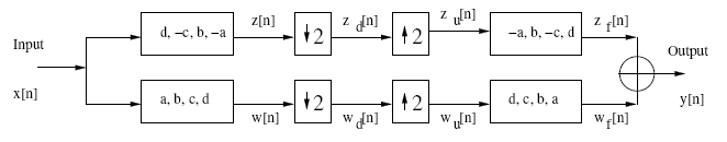
![$w[n]$](/RefArticleImages/AC20BF92F42FAE8F4B1DC1261E2AD45F_img9_9.gif) and
and ![$z[n]$](/RefArticleImages/AC20BF92F42FAE8F4B1DC1261E2AD45F_img10_9.gif) are just as they were earlier:
are just as they were earlier:![\begin{displaymath}w[n] = ax[n] + bx[n-1] + cx[n-2] + dx[n-3] \end{displaymath}](/RefArticleImages/AC20BF92F42FAE8F4B1DC1261E2AD45F_img108_9.gif)
![\begin{displaymath}z[n] = dx[n] - cx[n-1] + bx[n-2] - ax[n-3] . \end{displaymath}](/RefArticleImages/AC20BF92F42FAE8F4B1DC1261E2AD45F_img109_9.gif)
![$w[n-k]$](/RefArticleImages/AC20BF92F42FAE8F4B1DC1261E2AD45F_img189_9.gif) and
and ![$z[n-k]$](/RefArticleImages/AC20BF92F42FAE8F4B1DC1261E2AD45F_img190_9.gif) , are again found by
replacing
, are again found by
replacing  with
with  :
:
![\begin{displaymath}w[n-k] = ax[n-k] + bx[n-k-1] + cx[n-k-2] + dx[n-k-3] \end{displaymath}](/RefArticleImages/AC20BF92F42FAE8F4B1DC1261E2AD45F_img192_9.gif)
![\begin{displaymath}z[n-k] = dx[n-k] - cx[n-k-1] + bx[n-k-2] - ax[n-k-3] . \end{displaymath}](/RefArticleImages/AC20BF92F42FAE8F4B1DC1261E2AD45F_img193_9.gif)
![$w_d[n]$](/RefArticleImages/AC20BF92F42FAE8F4B1DC1261E2AD45F_img166_9.gif) and
and ![$z_d[n]$](/RefArticleImages/AC20BF92F42FAE8F4B1DC1261E2AD45F_img163_9.gif) , we again have to be careful about
whether
, we again have to be careful about
whether ![\begin{displaymath}w_d[n] = w[n], \;\; n\;\mathrm{is\;even} \end{displaymath}](/RefArticleImages/AC20BF92F42FAE8F4B1DC1261E2AD45F_img167_9.gif)
![\begin{displaymath}z_d[n] = z[n], \;\; n\;\mathrm{is\;even} \end{displaymath}](/RefArticleImages/AC20BF92F42FAE8F4B1DC1261E2AD45F_img168_9.gif)
![$w_u[n]$](/RefArticleImages/AC20BF92F42FAE8F4B1DC1261E2AD45F_img169_9.gif) and
and ![$z_u[n]$](/RefArticleImages/AC20BF92F42FAE8F4B1DC1261E2AD45F_img164_9.gif) must be treated with equal caution:
must be treated with equal caution:
![\begin{displaymath}w_u[n] = w_d[n] = w[n], \;\; n\;\mathrm{is\;even} \end{displaymath}](/RefArticleImages/AC20BF92F42FAE8F4B1DC1261E2AD45F_img170_9.gif)
![\begin{displaymath}w_u[n] = 0, \;\; n\;\mathrm{is\;odd} \end{displaymath}](/RefArticleImages/AC20BF92F42FAE8F4B1DC1261E2AD45F_img171_9.gif)
![\begin{displaymath}z_u[n] = z_d[n] = z[n], \;\; n\;\mathrm{is\;even} \end{displaymath}](/RefArticleImages/AC20BF92F42FAE8F4B1DC1261E2AD45F_img172_9.gif)
![\begin{displaymath}z_u[n] = 0, \;\; n\; \mathrm{is \; odd.} \end{displaymath}](/RefArticleImages/AC20BF92F42FAE8F4B1DC1261E2AD45F_img194_9.gif)
 , one of indices must be
even, while the other is odd. Likewise, if
, one of indices must be
even, while the other is odd. Likewise, if  ,
,  , etc.
The final signals of each channel are:
, etc.
The final signals of each channel are:
![\begin{displaymath}w_f[n] = d w_u[n] + c w_u[n-1] + b w_u[n-2] + a w_u[n-3] \end{displaymath}](/RefArticleImages/AC20BF92F42FAE8F4B1DC1261E2AD45F_img197_9.gif)
![\begin{displaymath}w_f[n] = d w[n] + 0 + b w[n-2] + 0, \;\; n\; \mathrm{is \; even} \end{displaymath}](/RefArticleImages/AC20BF92F42FAE8F4B1DC1261E2AD45F_img198_9.gif)
![\begin{displaymath}w_f[n] = 0 + c w[n-1] + 0 + a w[n-3], \;\; n\; \mathrm{is \; odd} \end{displaymath}](/RefArticleImages/AC20BF92F42FAE8F4B1DC1261E2AD45F_img199_9.gif)
![\begin{displaymath}z_f[n] = -a z_u[n] + b z_u[n-1] - c z_u[n-2] + d z_u[n-3] \end{displaymath}](/RefArticleImages/AC20BF92F42FAE8F4B1DC1261E2AD45F_img200_9.gif)
![\begin{displaymath}z_f[n] = -a z[n] + 0 - c z[n-2] + 0, \;\; n\; \mathrm{is \; even} \end{displaymath}](/RefArticleImages/AC20BF92F42FAE8F4B1DC1261E2AD45F_img201_9.gif)
![\begin{displaymath}z_f[n] = 0 + b z[n-1] + 0 + d z[n-3], \;\; n\; \mathrm{is \; odd.} \end{displaymath}](/RefArticleImages/AC20BF92F42FAE8F4B1DC1261E2AD45F_img202_9.gif)
![$y[n] = w_f[n] + z_f[n]$](/RefArticleImages/AC20BF92F42FAE8F4B1DC1261E2AD45F_img203_9.gif) :
:
![\begin{displaymath}y[n] = d w[n] + b w[n-2] - a z[n] - c z[n-2], \;\; n\; \mathrm{is \; even} \end{displaymath}](/RefArticleImages/AC20BF92F42FAE8F4B1DC1261E2AD45F_img204_9.gif)
![\begin{displaymath}y[n] = c w[n-1] + a w[n-3] + b z[n-1] + d z[n-3], \;\; n\; \mathrm{is \; odd.} \end{displaymath}](/RefArticleImages/AC20BF92F42FAE8F4B1DC1261E2AD45F_img205_9.gif)
![$y[n]$](/RefArticleImages/AC20BF92F42FAE8F4B1DC1261E2AD45F_img5_9.gif) in terms of
the original input
in terms of
the original input ![$x[n]$](/RefArticleImages/AC20BF92F42FAE8F4B1DC1261E2AD45F_img6_9.gif) :
:
![\begin{eqnarray*}
y[n] &=& d(a x[n] + b x[n-1] + c x[n-2] + d x[n-3]) \& & ...
...- c x[n-4] + b x[n-5] - a x[n-6]), \;\; n\; \mathrm{is \; odd.}
\end{eqnarray*}](/RefArticleImages/AC20BF92F42FAE8F4B1DC1261E2AD45F_img206_9.gif)
![\begin{eqnarray*}
y[n] &=& ad x[n] + bd x[n-1] + cd x[n-2] + dd x[n-3] \& &...
...cd x[n-4] + bd x[n-5] - ad x[n-6], \;\; n\; \mathrm{is \; odd.}
\end{eqnarray*}](/RefArticleImages/AC20BF92F42FAE8F4B1DC1261E2AD45F_img207_9.gif)
![\begin{eqnarray*}
y[n] &=& ac x[n-1] + bd x[n-1] \& & + aa x[n-3] + bb x[n-...
... \& & + ac x[n-5] + bd x[n-5], \;\; n\; \mathrm{is \; odd.}
\end{eqnarray*}](/RefArticleImages/AC20BF92F42FAE8F4B1DC1261E2AD45F_img208_9.gif)
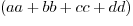
![\begin{eqnarray*}
y[n] &=& aa x[n-3] + bb x[n-3] + cc x[n-3] + dd x[n-3] \& & + ac x[n-1] + bd x[n-1] + ac x[n-5] + bd x[n-5] .
\end{eqnarray*}](/RefArticleImages/AC20BF92F42FAE8F4B1DC1261E2AD45F_img209_9.gif)
![$x[n-1]$](/RefArticleImages/AC20BF92F42FAE8F4B1DC1261E2AD45F_img119_9.gif) and
and ![$x[n-5]$](/RefArticleImages/AC20BF92F42FAE8F4B1DC1261E2AD45F_img120_9.gif) terms again, but that these
can be eliminated if we require
terms again, but that these
can be eliminated if we require  . Assuming this is the case,
we have our final expression for
. Assuming this is the case,
we have our final expression for ![\begin{displaymath}y[n] = (aa + bb + cc + dd) x[n-3] . \end{displaymath}](/RefArticleImages/AC20BF92F42FAE8F4B1DC1261E2AD45F_img211_9.gif)
 equals 1. When that is the case,
 ![$y[n] = x[n-3]$](/RefArticleImages/AC20BF92F42FAE8F4B1DC1261E2AD45F_img143_9.gif) , or
, or