Chapter 9.9 - Multiresolution
The above discussion is for a single pair of analysis filters. Multiresolution is the process of
taking the output from one channel
and putting it through another (or more) pair of analysis filters.
For the wavelet transform, we do this with the lowpass filter's output.
Wavelet packets, however, use an additional filter
pair for each channel.
We will examine multiresolution starting with the Daubechies four-coefficient
wavelet transform, with down-sampling and up-sampling, for two levels
of resolution (octaves), as shown in Figure 9.22.
Figure 9.22:
Two levels of resolution.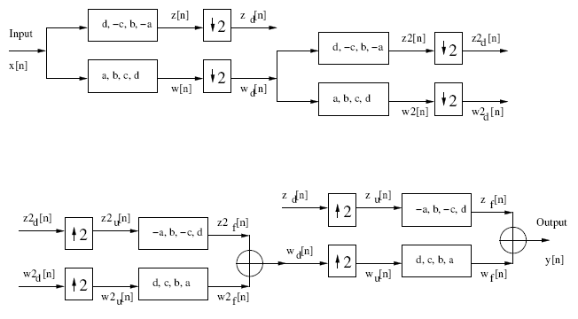 |
Signals ![$w[n]$](/RefArticleImages/AC20BF92F42FAE8F4B1DC1261E2AD45F_img9_9.gif) ,
, ![$w_d[n]$](/RefArticleImages/AC20BF92F42FAE8F4B1DC1261E2AD45F_img166_9.gif) ,
, ![$z[n]$](/RefArticleImages/AC20BF92F42FAE8F4B1DC1261E2AD45F_img10_9.gif) , and
, and ![$z_d[n]$](/RefArticleImages/AC20BF92F42FAE8F4B1DC1261E2AD45F_img163_9.gif) are the same as before.
are the same as before.
![\begin{displaymath}w[n] = ax[n] + bx[n-1] + cx[n-2] + dx[n-3] \end{displaymath}](/RefArticleImages/AC20BF92F42FAE8F4B1DC1261E2AD45F_img108_9.gif)
![\begin{displaymath}z[n] = dx[n] - cx[n-1] + bx[n-2] - ax[n-3] \end{displaymath}](/RefArticleImages/AC20BF92F42FAE8F4B1DC1261E2AD45F_img263_9.gif)
![\begin{displaymath}w_d[n] = w[n], \;\; n\; \mathrm{is \; even, 0\;otherwise} \end{displaymath}](/RefArticleImages/AC20BF92F42FAE8F4B1DC1261E2AD45F_img264_9.gif)
![\begin{displaymath}z_d[n] = z[n], \;\; n\; \mathrm{is \; even, 0\;otherwise} \end{displaymath}](/RefArticleImages/AC20BF92F42FAE8F4B1DC1261E2AD45F_img265_9.gif)
To generate ![$w2[n]$](/RefArticleImages/AC20BF92F42FAE8F4B1DC1261E2AD45F_img266_9.gif) ,
, ![$w2_d[n]$](/RefArticleImages/AC20BF92F42FAE8F4B1DC1261E2AD45F_img267_9.gif) ,
, ![$z2[n]$](/RefArticleImages/AC20BF92F42FAE8F4B1DC1261E2AD45F_img268_9.gif) , and
, and ![$z2_d[n]$](/RefArticleImages/AC20BF92F42FAE8F4B1DC1261E2AD45F_img269_9.gif) , we first
notice that they have the same relationship to as
and have to
, we first
notice that they have the same relationship to as
and have to ![$x[n]$](/RefArticleImages/AC20BF92F42FAE8F4B1DC1261E2AD45F_img6_9.gif) . In other words, we can reuse the above
equations, and replace with . Also, since there is a
down-sampler between and , every other value of
will be eliminated. Signal , by definition, is based upon ,
a down-sampled version of . Using the original
. In other words, we can reuse the above
equations, and replace with . Also, since there is a
down-sampler between and , every other value of
will be eliminated. Signal , by definition, is based upon ,
a down-sampled version of . Using the original  , therefore, means
that we must say that every other value from the even values of
will be eliminated. In other words, the only values that will get
through the second down-sampler are the ones where is evenly divisible
by 4.
, therefore, means
that we must say that every other value from the even values of
will be eliminated. In other words, the only values that will get
through the second down-sampler are the ones where is evenly divisible
by 4.
![\begin{displaymath}w2[n] = a w_d[n] + b w_d[n-1] + c w_d[n-2] + d w_d[n-3] \end{displaymath}](/RefArticleImages/AC20BF92F42FAE8F4B1DC1261E2AD45F_img270_9.gif)
![\begin{displaymath}z2[n] = d w_d[n] - c w_d[n-1] + b w_d[n-2] - a w_d[n-3] \end{displaymath}](/RefArticleImages/AC20BF92F42FAE8F4B1DC1261E2AD45F_img271_9.gif)
![\begin{displaymath}w2_d[n] = w2[n], \;\; n\;\mathrm{is\;divisible\;by\;4} \end{displaymath}](/RefArticleImages/AC20BF92F42FAE8F4B1DC1261E2AD45F_img272_9.gif)
![\begin{displaymath}z2_d[n] = z2[n], \;\; n\;\mathrm{is\;divisible\;by\;4} \end{displaymath}](/RefArticleImages/AC20BF92F42FAE8F4B1DC1261E2AD45F_img273_9.gif)
Looking now at the reconstruction (synthesis) part, ![$w2_u[n]$](/RefArticleImages/AC20BF92F42FAE8F4B1DC1261E2AD45F_img274_9.gif) and
and ![$z2_u[n]$](/RefArticleImages/AC20BF92F42FAE8F4B1DC1261E2AD45F_img275_9.gif) are up-sampled versions of and . We have to keep track of
values of that are divisible by 4, and also values of that are
even, but not divisible by 4, such as the number 6. Since we have taken
a signal where all of the index terms are already even, the function
of the down-sampler followed by the up-sampler is that the "even-even'
(divisible by 4)
indices are kept, but the "odd-even' indices (divisible by 2, but
not divisible by 4, such as 2, 6, 10, etc.)
are eliminated, then made to zero by the up-sampler.
are up-sampled versions of and . We have to keep track of
values of that are divisible by 4, and also values of that are
even, but not divisible by 4, such as the number 6. Since we have taken
a signal where all of the index terms are already even, the function
of the down-sampler followed by the up-sampler is that the "even-even'
(divisible by 4)
indices are kept, but the "odd-even' indices (divisible by 2, but
not divisible by 4, such as 2, 6, 10, etc.)
are eliminated, then made to zero by the up-sampler.
![\begin{displaymath}w2_u[n] = w2_d[n] = w2[n], \;\; n\; \mathrm{is\;even}\texttt{-}\mathrm{even} \end{displaymath}](/RefArticleImages/AC20BF92F42FAE8F4B1DC1261E2AD45F_img276_9.gif)
![\begin{displaymath}w2_u[n] = 0, \;\; n\; \mathrm{is\;odd}\texttt{-}\mathrm{even} \end{displaymath}](/RefArticleImages/AC20BF92F42FAE8F4B1DC1261E2AD45F_img277_9.gif)
![\begin{displaymath}w2_u[n] \; \mathrm{is\;undefined, \; otherwise} \end{displaymath}](/RefArticleImages/AC20BF92F42FAE8F4B1DC1261E2AD45F_img278_9.gif)
![\begin{displaymath}z2_u[n] = z2_d[n] = z2[n], \;\; n\; \mathrm{is\;even}\texttt{-}\mathrm{even} \end{displaymath}](/RefArticleImages/AC20BF92F42FAE8F4B1DC1261E2AD45F_img279_9.gif)
![\begin{displaymath}z2_u[n] = 0, \;\; n\; \mathrm{is\;odd}\texttt{-}\mathrm{even} \end{displaymath}](/RefArticleImages/AC20BF92F42FAE8F4B1DC1261E2AD45F_img280_9.gif)
![\begin{displaymath}z2_u[n] \; \mathrm{is\;undefined, \; otherwise} \end{displaymath}](/RefArticleImages/AC20BF92F42FAE8F4B1DC1261E2AD45F_img281_9.gif)
Signals ![$w2_f[n]$](/RefArticleImages/AC20BF92F42FAE8F4B1DC1261E2AD45F_img282_9.gif) and
and ![$z2_f[n]$](/RefArticleImages/AC20BF92F42FAE8F4B1DC1261E2AD45F_img283_9.gif) are found as before:
are found as before:
![\begin{displaymath}w2_f[n] = d w2_u[n] + c w2_u[n-1] + b w2_u[n-2] + a w2_u[n-3] \end{displaymath}](/RefArticleImages/AC20BF92F42FAE8F4B1DC1261E2AD45F_img284_9.gif)
![\begin{displaymath}w2_f[n] = d w2[n] + 0 + b w2[n-2] + 0, \;\; n\; \mathrm{is\;even}\texttt{-}\mathrm{even} \end{displaymath}](/RefArticleImages/AC20BF92F42FAE8F4B1DC1261E2AD45F_img285_9.gif)
![\begin{displaymath}w2_f[n] = 0 + c w2[n-1] + 0 + a w2[n-3], \;\; n\; \mathrm{is\;odd}\texttt{-}\mathrm{even} \end{displaymath}](/RefArticleImages/AC20BF92F42FAE8F4B1DC1261E2AD45F_img286_9.gif)
![\begin{displaymath}z2_f[n] = -a z2_u[n] + b z2_u[n-1] - c z2_u[n-2] + d z2_u[n-3] \end{displaymath}](/RefArticleImages/AC20BF92F42FAE8F4B1DC1261E2AD45F_img287_9.gif)
![\begin{displaymath}z2_f[n] = -a z2[n] + 0 - c z2[n-2] + 0, \;\; n\; \mathrm{is\;even}\texttt{-}\mathrm{even} \end{displaymath}](/RefArticleImages/AC20BF92F42FAE8F4B1DC1261E2AD45F_img288_9.gif)
![\begin{displaymath}z2_f[n] = 0 + b z2[n-1] + 0 + d z2[n-3], \;\; n\; \mathrm{is\;odd}\texttt{-}\mathrm{even.} \end{displaymath}](/RefArticleImages/AC20BF92F42FAE8F4B1DC1261E2AD45F_img289_9.gif)
We can finish the reconstruction for the second octave by looking
at the result when and are added together to recreate
. We will call this recreated signal ![$w_d[n]'$](/RefArticleImages/AC20BF92F42FAE8F4B1DC1261E2AD45F_img290_9.gif) , until we are
certain that it is the same as .
, until we are
certain that it is the same as .
![\begin{displaymath}w_d[n]' = w2_f[n] + z2_f[n] \end{displaymath}](/RefArticleImages/AC20BF92F42FAE8F4B1DC1261E2AD45F_img291_9.gif)
![\begin{displaymath}w_d[n]' = d w2[n] + b w2[n-2] - a z2[n] - c z2[n-2], \;\; n\; \mathrm{is\;even}\texttt{-}\mathrm{even} \end{displaymath}](/RefArticleImages/AC20BF92F42FAE8F4B1DC1261E2AD45F_img292_9.gif)
![\begin{displaymath}w_d[n]' = c w2[n-1] + a w2[n-3] + b z2[n-1] + d z2[n-3], \;\; n\; \mathrm{is\;odd}\texttt{-}\mathrm{even} \end{displaymath}](/RefArticleImages/AC20BF92F42FAE8F4B1DC1261E2AD45F_img293_9.gif)
The important thing to do here is to show that the two signals marked
in Figure 9.22 are exactly the same. This means
finding the previous expression in terms of only.
First, we will take the
expressions for and , and find ![$w2[n-k]$](/RefArticleImages/AC20BF92F42FAE8F4B1DC1261E2AD45F_img294_9.gif) and
and ![$z2[n-k]$](/RefArticleImages/AC20BF92F42FAE8F4B1DC1261E2AD45F_img295_9.gif) .
.
![\begin{displaymath}w2[n-k] = a w_d[n-k] + b w_d[n-k-1] + c w_d[n-k-2] + d w_d[n-k-3] \end{displaymath}](/RefArticleImages/AC20BF92F42FAE8F4B1DC1261E2AD45F_img296_9.gif)
![\begin{displaymath}z2[n-k] = d w_d[n-k] - c w_d[n-k-1] + b w_d[n-k-2] - a w_d[n-k-3] \end{displaymath}](/RefArticleImages/AC20BF92F42FAE8F4B1DC1261E2AD45F_img297_9.gif)
Now, we can plug these into the previous expressions.
![\begin{eqnarray*}
w_d[n]' &=& d (a w_d[n] + b w_d[n-1] + c w_d[n-2] + d w_d[n-3...
... a w_d[n-6]), \;\; n \; \mathrm{is\;odd}\texttt{-}\mathrm{even}
\end{eqnarray*}](/RefArticleImages/AC20BF92F42FAE8F4B1DC1261E2AD45F_img298_9.gif)
Rewriting these expressions and lining them up into columns gives us:
is even-even:
![\begin{displaymath}
\begin{array}{ccccc}
w_d[n]' = & & & & \ad w_d[n] & +\; ...
...] & -\; bc w_d[n-4] \+\; ac w_d[n-5]. & & & &
\end{array} \end{displaymath}](/RefArticleImages/AC20BF92F42FAE8F4B1DC1261E2AD45F_img299_9.gif)
is odd-even:
![\begin{displaymath}
\begin{array}{ccccc}
w_d[n]' = & & & & \ac w_d[n-1] & +\;...
...4] & +\; bd w_d[n-5] \-\; ad w_d[n-6]. & & & &
\end{array} \end{displaymath}](/RefArticleImages/AC20BF92F42FAE8F4B1DC1261E2AD45F_img300_9.gif)
Canceling out terms gives us:
is even-even:
![\begin{displaymath}
\begin{array}{cccc}
w_d[n]' = & bd w_d[n-1] & +\; dd w_d[n-3...
...-3] & \& & +\; cc w_d[n-3] & +\; ac w_d[n-5] .
\end{array} \end{displaymath}](/RefArticleImages/AC20BF92F42FAE8F4B1DC1261E2AD45F_img301_9.gif)
is odd-even:
![\begin{displaymath}
\begin{array}{cccc}
w_d[n]' = & ac w_d[n-1] & +\; cc w_d[n-3...
...-3] & \& & +\; dd w_d[n-3] & +\; bd w_d[n-5] .
\end{array} \end{displaymath}](/RefArticleImages/AC20BF92F42FAE8F4B1DC1261E2AD45F_img302_9.gif)
Examining the above equations, we see that we have the same expression
for when is even-odd as when it is even-even. Therefore, we can
rewrite the above expression, with the note that must be even.
We know from the previous section that  , so the terms with
![$w_d[n-1]$](/RefArticleImages/AC20BF92F42FAE8F4B1DC1261E2AD45F_img303_9.gif) and
and ![$w_d[n-5]$](/RefArticleImages/AC20BF92F42FAE8F4B1DC1261E2AD45F_img304_9.gif) will cancel out. This leaves us with
will cancel out. This leaves us with
![$w_d[n]' = (aa + bb + cc + dd) w_d[n-3]$](/RefArticleImages/AC20BF92F42FAE8F4B1DC1261E2AD45F_img305_9.gif) . As previously noted,
. As previously noted,
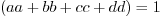 , so we get the final expression for
![$w_d[n]' = w_d[n-3]$](/RefArticleImages/AC20BF92F42FAE8F4B1DC1261E2AD45F_img307_9.gif) . The reconstructed is the same as a
delayed version of the original . This is no surprise, since
we have simply inserted a copy of the 1-octave filter bank structure between
the original and the reconstruction. When we looked at the
filter bank structure for 1-octave, we saw that the result
. The reconstructed is the same as a
delayed version of the original . This is no surprise, since
we have simply inserted a copy of the 1-octave filter bank structure between
the original and the reconstruction. When we looked at the
filter bank structure for 1-octave, we saw that the result ![$y[n]$](/RefArticleImages/AC20BF92F42FAE8F4B1DC1261E2AD45F_img5_9.gif) was a
delayed version of .
was a
delayed version of .
The next step is to take the reconstructed signal, , and recombine
it with to get . Note that in the analysis
(top part) of Figure 9.22 and the in the synthesis
(bottom part) of this figure must be exactly the same.
But we saw above that they are not exactly the same, since is
a delayed version of .
We can deal with this in a couple of
ways. If we are designing hardware to perform the wavelet transform,
we can simply add three (that is, length of filter ) delay units to
channel with the signal. If we are writing software to do this, we can
put three zeros before , or we could shift forward by three
positions, getting rid of the first three values.
The important thing is that and are
properly aligned. We will assume that this second method has been used
to "correct' to be exactly equal to . If we were
to use the first method of delaying , then the output would
be reconstructed using
) delay units to
channel with the signal. If we are writing software to do this, we can
put three zeros before , or we could shift forward by three
positions, getting rid of the first three values.
The important thing is that and are
properly aligned. We will assume that this second method has been used
to "correct' to be exactly equal to . If we were
to use the first method of delaying , then the output would
be reconstructed using ![$w_d[n-3]$](/RefArticleImages/AC20BF92F42FAE8F4B1DC1261E2AD45F_img309_9.gif) and
and ![$z_d[n-3]$](/RefArticleImages/AC20BF92F42FAE8F4B1DC1261E2AD45F_img310_9.gif) , implying that the
output would be delayed by an additional three units. That is, instead
of having
, implying that the
output would be delayed by an additional three units. That is, instead
of having ![$y[n] = x[n-3]$](/RefArticleImages/AC20BF92F42FAE8F4B1DC1261E2AD45F_img143_9.gif) as the result,
we would have
as the result,
we would have
![$y[n] = x[n-3-3] = x[n-6]$](/RefArticleImages/AC20BF92F42FAE8F4B1DC1261E2AD45F_img311_9.gif) .
.
Tracing the path of and is very similar to that of
and .
![\begin{displaymath}w_u[n] = w_d[n] = w[n], \;\; n\;\mathrm{is\;even} \end{displaymath}](/RefArticleImages/AC20BF92F42FAE8F4B1DC1261E2AD45F_img170_9.gif)
![\begin{displaymath}w_u[n] = 0, \;\; n\;\mathrm{is\;odd} \end{displaymath}](/RefArticleImages/AC20BF92F42FAE8F4B1DC1261E2AD45F_img171_9.gif)
![\begin{displaymath}z_u[n] = z_d[n] = z[n], \;\; n\;\mathrm{is\;even} \end{displaymath}](/RefArticleImages/AC20BF92F42FAE8F4B1DC1261E2AD45F_img172_9.gif)
![\begin{displaymath}z_u[n] = 0, \;\; n\;\mathrm{is\;odd} \end{displaymath}](/RefArticleImages/AC20BF92F42FAE8F4B1DC1261E2AD45F_img173_9.gif)
Notice that the "otherwise' case has been dropped, since is either
odd or even. Finding ![$w_f[n]$](/RefArticleImages/AC20BF92F42FAE8F4B1DC1261E2AD45F_img180_9.gif) and
and ![$z_f[n]$](/RefArticleImages/AC20BF92F42FAE8F4B1DC1261E2AD45F_img165_9.gif) is just like finding
and :
is just like finding
and :
![\begin{displaymath}w_f[n] = d w_u[n] + c w_u[n-1] + b w_u[n-2] + a w_u[n-3] \end{displaymath}](/RefArticleImages/AC20BF92F42FAE8F4B1DC1261E2AD45F_img197_9.gif)
![\begin{displaymath}w_f[n] = d w[n] + 0 + b w[n-2] + 0, \;\; n\; \mathrm{is \; even} \end{displaymath}](/RefArticleImages/AC20BF92F42FAE8F4B1DC1261E2AD45F_img198_9.gif)
![\begin{displaymath}w_f[n] = 0 + c w[n-1] + 0 + a w[n-3], \;\; n\; \mathrm{is \; odd} \end{displaymath}](/RefArticleImages/AC20BF92F42FAE8F4B1DC1261E2AD45F_img199_9.gif)
![\begin{displaymath}z_f[n] = -a z_u[n] + b z_u[n-1] - c z_u[n-2] + d z_u[n-3] \end{displaymath}](/RefArticleImages/AC20BF92F42FAE8F4B1DC1261E2AD45F_img200_9.gif)
![\begin{displaymath}z_f[n] = -a z[n] + 0 - c z[n-2] + 0, \;\; n\; \mathrm{is \; even} \end{displaymath}](/RefArticleImages/AC20BF92F42FAE8F4B1DC1261E2AD45F_img201_9.gif)
![\begin{displaymath}z_f[n] = 0 + b z[n-1] + 0 + d z[n-3], \;\; n\; \mathrm{is \; odd.} \end{displaymath}](/RefArticleImages/AC20BF92F42FAE8F4B1DC1261E2AD45F_img202_9.gif)
Adding to produces , just as we saw for the
single-octave case. The important thing to notice is that the
reconstruction is exactly the same as the single-octave case,
provided that is exactly the same in both the analysis and synthesis (top and bottom)
parts of Figure 9.22.
Here we have seen that we can make the filter bank structure
work recursively, and still get a perfectly reconstructed signal. While
this section uses only two levels of recursion (octaves), it
should be clear that we can use as many octaves as we want. The only
limitation is that imposed by the length of the input signal, since
every octave uses half the number of inputs as the octave above it.
In other words, exists only for even values of the index ,
while the input signal has values for even and odd values of .
If has 16 samples, then would have 8, and would
have 4, etc.
© 2026 Infinity Science Press