Orbital Mechanics, Third Edition

In Chapter 8, the physical phenomena of orbit perturbations due to various sources have been discussed. This chapter provides an introduction to the mathematical foundations of those perturbations and the various methods of solution.
Before going into equations of motion for orbit perturbations, it is important to review the two-body equations of motion in relative form. The equations of motion for a satellite moving under the attraction of a point mass planet without any other perturbations can be given in the planet-centered coordinates as
| (9.1) | |
where
| r | = position vector of the satellite |
| ? | = gravitational constant |
| t | = time |
Equation (9.1) is a set of three simultaneous second-order nonlinear differential equations. There are six constants of integration. The solution of Eq. (9.1) can be either in terms of initial position and velocity:
; or in terms of the six orbit elements: a, e, i, ?, ?, M.
The closed-form conic solutions of the two-body equations of motion have been given in the earlier chapters, and they may be expressed in a general functional form as
| (9.2) | |
or
| (9.3) | |
Five of the six orbit elements ( a ? ?) in the preceding expression are constants, and M is the mean anomaly defined by
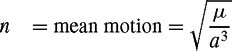
| (9.4) | |
where
| M 0 | = mean anomaly at epoch, t 0 |
| |
Figure 9.1 shows the orbit geometry of an orbiting satellite in the inertial Earth-centered equatorial coordinate system (ECI). It is important to know...