B.1 Principal Invariants

Given any second-order Cartesian tensor a with components expressed as

(B.1)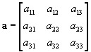

the principal values of a, denoted as a ₁, a ₂, and a ₃, may be computed from the solution of the eigenproblem

(B.2)

in which the (right) eigenvectors q ^{( m )} denote principal directions for the associated eigenvalue a _m. Non-trivial solutions of Eq. (B.2) require

(B.3)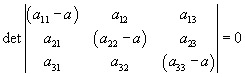

Expanding the determinant results in the cubic equation

(B.4)

where:

(B.5)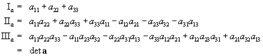

The quantities I _a, II _a, and III _a are called the principal invariants of a. The roots of Eq. (B.4) give the principal values a _m.

The invariants for the deviator of a may be obtained by using

(B.6)

where a is the mean defined as

(B.7)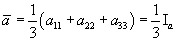

Substitution of Eq. (B.6) into Eq. (B.2) gives

(B.8)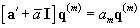

or

(B.9)

which yields a cubic equation for principal values of the deviator given as

(B.10)

where invariants of a ? are denoted as , , and .

Since the deviators a ? differ from the total a by a mean term only, we observe from Eq. (B.9) that the directions of their principal values coincide, and the three principal values are related through

(B.11)

Moreover Eq. (B.10) generally has a closed-form solution which may be constructed by using the Cardon formula.1 ^,2

The definition of a ? given by Eq. (B.6) yields

(B.12)

Using this result,...