Overview

It is always useful to have limiting analytical solutions to any theory. In this chapter LGT is solved analytically in the strong-coupling limit where the constant ? in the action becomes very small. Thus we are here interested in the following limit of the theory

(34.1)

From Eq. (33.32), for example, for in d=4 dimensions, . Small ? corresponds to large g ²; hence the name strong-coupling limit. References [Wi74, Cr83, Ko83] provide basic background here; this section is based on [It89].

Since the action appears in the exponent of the statistical operator, small ? is equivalent to high temperature in the usual partition function in statistical mechanics. One can think of 1/ ? ? T _eff as an effective temperature here. If we recall the plot of the magnetization m ⁴ vs ? _C/ ? in Fig. 30.6 and Prob. 32.2, then the strong-coupling limit corresponds to the far right hand side of the figure.

Basic Observation: In the limit ??0, one can expand the exponential of the action in the statistical operator and keep the first nonvanishing term in a power series in ?.

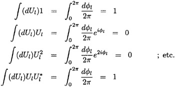
Let us start with U(1) and then generalize. This calculation is readily carried out because the path integral over the individual link variables takes a very simple form

(34.2)

As a ?0 one can write

(34.3)

Here C indicates the contour of the Wilson loop (Fig.