2.2 Transfer Functions

Let us consider a system governed by the following differential equation:

Assume that the initial conditions are equal to zero, and denote and by Y ( s) and U ( s), respectively. The Laplace transform of (2.5) yields:

This Laplace transform represents the transfer function of the system considered. The roots of the numerator of the transfer function represent the zeros (transmission zeros) of the system, while the roots of the denominator represent the poles (natural modes). Equation (2.6) may be written as follows:

where:

and "*" represents the convolution. ^[3] The order ^[4] of the system corresponds to the highest power of s in the denominator of the transfer function. The transfer function is a useful tool for representing the behavior of a system or of a set of systems in series, in parallel or in feedback. Let us consider the following cases:

1. N systems in series (see Figure 2.1). We obtain:

   
   Figure 2.1: Systems in series

   
   

   The Laplace transform of the global output Y ( s) is equal to:

   
   

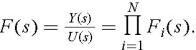
   and the equivalent transfer function is:

   
   

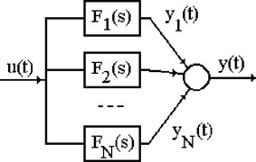
2. N systems in parallel (see Figure 2.2). We obtain:

   
   

   
   Figure 2.2: Systems in parallel

   and

   
   

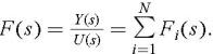
   which implies:

   
   

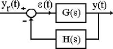
3. A feedback system (see Figure 2.3). The equations governing the behavior of this system are:

   
   

   
   Figure 2.3: Feedback system

   which yields the closed-loop transfer function:

   
   

   where T ( s) = G ( s) H (