2.4 Differential and Integral Equations

Problem 2.14

Solve the following differential equation:

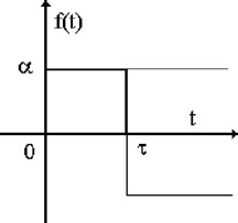
where f ( t) is plotted in Figure 2.7.

Figure 2.7: The function f ( t)

Solution 2.14

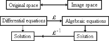
The use of Laplace transforms for solving differential equations is illustrated by the diagram in Figure 2.8.

Figure 2.8: The Laplace transform as a tool for solving differential equations

Let us decompose the function f ( t) into elementary functions:

where 1 ( t) represents the unit step. The Laplace transform of Equation (2.12) yields:

Let us consider the following Laplace transform:

which implies ^[11]:

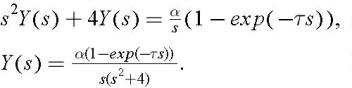
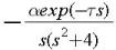
The inverse Laplace transform of:

is

Finally, we obtain:

Problem 2.15

Solve the following differential equation:

Solution 2.15

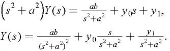
The Laplace transform yields:

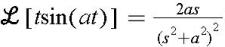
Recall that:

and

Therefore,

and

Finally, we obtain:

Problem 2.16

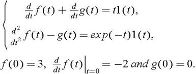
For t > 0, solve the following system of differential equations:

Observe that we have introduced the unit step 1( t) because the Laplace transform is defined for functions equal to zero for t < 0.

Solution 2.16

We calculate the following Laplace transforms:

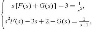
Transforming the system of differential equations, we obtain a system of equations where the unknowns are the Laplace transforms F ( s) and G ( s):

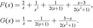
For Re ( s) > 0, we derive the partial fraction expansions:

Finally, the solution of the system of differential equations is obtained by taking the inverse Laplace transform: