5.4 Finite-Element and Finite-Difference Methods

Finite-element and finite-difference methods have only been applied in the case of the ?-independent TM and TE modes. The field equations for those modes can be easily obtained by putting m = 0 in (5.16) and (5.41), respectively. It is customary, however, to express the field components of the TM (TE) modes in terms of H _? (E _?), rather than ? ^e ( ? ^h). Hence, in the TM case we have, from (5.15) and (5.16),

(5.95a)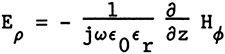

(5.95b)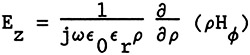

(5.95c)

where we defined for future reference operator D as

(5.96)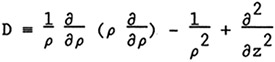

The equations (5.95) are valid in each region over which ? _r is constant, but do not hold at interfaces across which ? _r changes discontinuously [27]. However, we may solve for the fields in each homogeneous region and match the tangential components at the interfaces to obtain a solution that is valid everywhere.

In the TE case, we have, from (5.40) and (5.41),

(5.97a)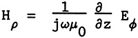

(5.97b)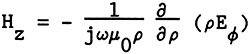

and

(5.97c)

In the remainder of this section we will limit attention to the TE case, since the development for the TM case is similar.

In the finite-element method [28,29], the resonator cross section (Fig. 5.1) is subdivided into a finite number of patches or "finite elements," usually of triangular shape, and in each patch the unknown is represented as a linear combination of interpolatory polynomials N _i. Hence, if we put ? = E _? for notational simplicity,...