Chapter List

Overview

If we have a differential equation that we cannot solve analytically then we can always try to treat the problem numerically. In this chapter we consider one numerical way to approximate the equation

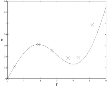
The first step is to give up the idea of finding a solution for all values of the independent variable ( x( t) for any t ? ) and instead try to find an approximation to the solution at a discrete set of values of t. This is illustrated in Figure 21.1.

Fig. 21.1: The curve shows a notional true solution , and the crosses show the result of numerically approximating the solution at a discrete set of values of t.

In the simplest case we try to approximate the solution at equally spaced values of the independent variable. This means, for example, that we want to approximate x( h), x(2 h), x(3 h), x(4 h), etc. The difference between two successive times, here h, is called the timestep (or more generally, when the independent variable is not necessarily time, the step size).

If we have a method for approximating x( t + h) given x( t), then we can apply the method repeatedly to find approximations for x( nh) for any n, if