We saw at the very end of the last chapter that the most complicated dynamics that can occur in a system of two coupled equations (a two-dimensional system) is a periodic orbit.

In this chapter we discuss, briefly, a three-dimensional system of equations, the Lorenz equations, which demonstrates that much more complexity is possible once we have three variables. Without the help of numerical solutions and computer-aided visualisation our understanding of these equations would still be poor. This chapter contains many computer-generated images, and some samples of MATLAB output performing some tedious eigenvalue calculations. Most of this was generated by the M-file lorenz37.m, and it might be helpful to have this program running as you read.

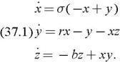
Lorenz introduced his relatively simple system as a model in which to study various theoretical problems involved in meteorology, and in particular in weather prediction. ^[1] It is based on a model of convection (when a layer of fluid is heated from below), greatly simplified. The model is

There are three parameters in the problem: b, r, and ?. Standard values have established themselves over the years: b = 8 /3, r = 28, and ? = 10.

% parameters>> sigma=10; r=28; b=8/3;

The basic steps towards understanding the problem should be familiar from our analysis of two-dimensional systems; we find the stationary points and determine their stability.

For these parameter values there are three stationary points; one at the origin (it is easy to find...