An Introduction to Ordinary Differential Equations
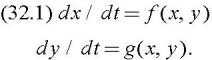
We now turn our attention to coupled nonlinear systems. We will concentrate on autonomous systems in which the right-hand side does not depend explicitly on time,
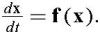
Using the vector notation x = ( x, y) and f( x) = ( f (x, y), g(x, y)), this equation can be rewritten
Our approach will be to try to understand the dynamics of these equations (the behaviour of their solutions) in a qualitative way by drawing the phase diagram in the ( x, y) plane ( the phase plane ), just as we have done for linear equations in the past three chapters. We will find that we can piece together the phase por trait for nonlinear systems from a collection of phase portraits for linear (or near ly linear) systems near the stationary points.
A stationary point is a point ( x* , y*) at which
=
= 0, i.e. where
Because solutions are unique, it follows that if ( x* , y*) is a stationary point then solutions starting at ( x* , y*) remain there for all time. The phase portraits we drew in the previous chapters were fairly simple, since we only ever had a single stationary point at the origin.
Our phase portraits will show the stationary points marked by crosses, and include a representative collection of trajectories (the curves traced out by solutions as they change in time) with the...