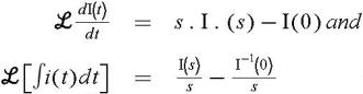
Network Analysis & Circuits

The Laplace transform is a very important mathematical tool. By using the Laplace transform, any electrical circuit can be solved and calculations are very easy for transient and steady state conditions. The following steps involve the analysis of a linear system (electrical or mechanical, etc.). In this chapter we will consider only the electrical system.
Apply KVL and make a differential or integro-differential equation form.
Take the Laplace transform of the system differential or integro-differential equation together with the input excitation to obtain an algebraic equation in the s-domain.
Now take the Laplace inverse transform to get the solution in the time domain.
In the last chapter we discussed
and the Laplace transform of second order or higher. These formulas are very important to solve a linear differential equation. Now consider a second differential equation
We know,
and
Taking the Laplace transform on both sides of Equation (7.1),
where I(0) = value of i(t) at t = 0
Now taking the Laplace inverse,
The result, as in Equation (7.5), not only depends on the characteristic roots but also on the excitation function and initial conditions. The Laplace inverse of Equation (7.5) gives the time response, if we can modify the right-hand side of Equation (7.5) to a known form of the available Laplace inverse transform and convert the response in the time domain.
Solve the differential equation
and
Solution: Taking the Laplace transform, ![]()
Now taking the partial fraction,