3.1 INTRODUCTION AND DEFINITIONS

A random process may be viewed as a collection of random variables, with time t as a parameter running through all real numbers. In Chapter 1, we defined a random variable as a mapping of the elements of the sample space S into points of the real axis. For random processes, the sample space would map into a family of time functions. Formally, we say a random process X( t) is a mapping of the elements of the sample space into functions of time. Each element of the sample space is associated with a time function as shown in Figure 3.1.

Figure 3.1: Mapping of sample space into sample functions.

Associating a time function to each element of the sample space results in a family of time functions called the ensemble. Hence, the ensemble is the set of sample functions with the associated probabilities. Observe that we are denoting the random process by X( t), and not X( t, ?), where the dependence on ? is omitted. A sample function is denoted by x( t).

Example 3.1

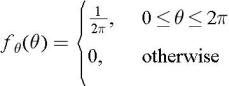
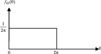
Consider a random process X( t) = A cos( ? t + ?), where ? is a random variable uniformly distributed between 0 and 2 ?, as shown in Figure 3.2. That is,

Figure 3.2: Density function of ?.

some sample functions of this random process are shown...