2.2.1 General remarks

We consider the discretization of Eq. (2.12) with

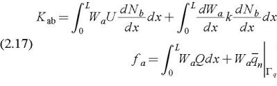
where N _a are shape functions and represents a set of still unknown parameters. Here we shall take these to be the nodal values of ?. The weighted residual form of the one-dimensional problem is written as (see Chapter 1)

Integrating the second term by parts gives

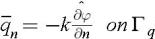
where

and

is assumed. For a typical internal node a' the approximating equation becomes

where

and the domain of the problem is 0 ? x ? L.

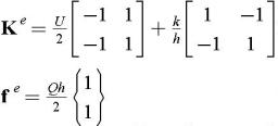
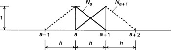
For linear shape functions (Fig. 2.1), Galerkin weighting ( W _a = N _a) and elements of equal size h, wehavefor constant values of U, k and Q (see Appendix D)

Figure 2.1: A linear shape function for a one-dimensional problem.

which yields a typical assembled equation (after multiplying by h/ k) for node a

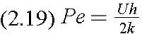
where

is the element Peclet number. Incidentally, for the case of constant Q the above is identical to the usual central finite difference approximation obtained by putting (for node a)

and

The algebraic equations (2.18) are obviously non-symmetric and their accuracy deteriorates as the parameter Pe increases i.e. when convective terms are of primary importance. Indeed as Pe ? ?, the solution is purely oscillatory and bears no relation to the underlying problem. This may be ascertained by considering Eq. (2.18) for...