2.5.1 Mathematical background
The objective of this section is to develop procedures of general applicability for the solution by direct time-stepping methods of Eq. (2.1) written for scalar values of ?, F iand G i. Starting from the scalar form of Eq. (2.4)
though consideration of the procedure for dealing with a vector-valued function is included in Appendix E. To allow a simple interpretation of the various methods and of behaviour patterns the scalar equation in one dimension in non-conservation form [see Eq. (2.11)], i.e.
will be considered. The problem so defined is non-linear unless U is independent of ?. However, the non-conservative equation (2.75) admits a spatial variation of U and is quite general.
In the general form (2.74) the main behaviour patterns can be determined by a change of the independent variable x to x ? such that
Noting that for ? = ?( x ?, t) we have
The one-dimensional equation (2.75) now becomes simply
and equations of this type can be readily discretized with self-adjoint spatial operators and solved by standard Galerkin finite element procedures. [1]
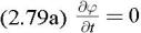
The coordinate system of Eq. (2.76) describes characteristic directions and the moving nature of the coordinates must be noted. A further corollary of the coordinate change is that with no conduction or source terms, i.e. when k = 0 and Q = 0, we have simply
or, for the one-dimensional...

 TABLE OF CONTENTS