3.7 Two-dimensional filtering (areal filtering)

Two-dimensional filtering has two spatial dimensions instead of one, yet it is sometimes wrongly called 3D filtering. As with digital sampling, the 2D filtering has cross terms that are not seen easily from profile filtering. The filtering action is that of convolution, which has already been mentioned in the space domain corresponding to multiplication in the frequency domain. In this case, the window or weighting function itself has two spatial dimensions x and y as indicated in Figure 3.51.

Figure 3.51: Areal sampling

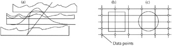
To get best results, the weighting function boundary shape should be as close as possible to the lay pattern. This is a constraint but it is only weak because the convolution can take place anyway. Ideally, for manufacturing the weighting function, it should have some connection with the path of the tool.

The basic equation for the 2D spectrum is F( w,v)

(3.25)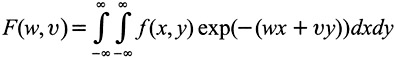

and the autocorrelation

(3.26)

The main thing to remember is that there are two spatial axes x and y. This is not to be confused with the two variables in the Wigner distribution. In these, one of the variables is spatial x, one is frequency w i.e. only one spatial variable. The problem is that the 'space frequency' functions are plotted against two axes in exactly the same way as the areal (3D) autocorrelation but the information is still about the profile and not the areal surface.

In summary, two-dimensional filtering gives more information...