Logic-Timing Simulation and the Degradation Delay Model

Chapter 3: Degradation and Inertial Effects

Manuel Jes s Bellido D az David Guerrero Martos

3.1 Introduction

In the previous chapter we have seen the main issues of digital circuit time modelling. In order to enhance the precision of a delay model it is necessary to take into account most of the effects related to the behaviour of real digital components. In this chapter we will introduce and model the so-called degradation effect which, as will be shown, is related to the inertial effect.

3.1.1 Degradation and Inertial Effects

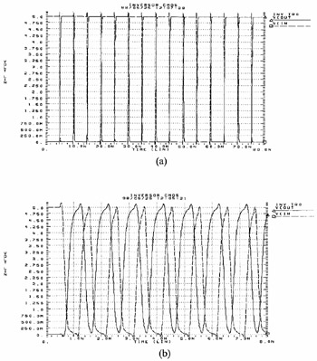
When the propagation delay of the circuit is much shorter than the period corresponding to its operation frequency, signals and gates may be considered ideal, that is, with zero delay and transition time (Fig. 3.1 (a)). Also, in this case it is acceptable to suppose that each transition is not affected by the previous one. Having said that, as operation frequency increases, non-ideal effects ( i.e. effects observed in non-ideal gates) become more relevant. For example, in Fig. 3.1 (b) we can see two non-ideal effects: there is a non-zero propagation delay and signal transitions are not instantaneous.


Figure 3.1: Digital signal shape, a) Delay/Signal Period = 0.01 b) Delay/Signal Period = 0.1.

Thus, because of the rising operation speed of the circuits, it becomes increasingly important to include non-ideal effects in the delay models used for timing analysis. In this chapter we will introduce and model the so-called degradation effect [Juan et al. (1997a)]. At the beginning, because of the low operation frequency, these effects...

UNLIMITED FREE
ACCESS
TO THE WORLD'S BEST IDEAS

SUBMIT
Already a GlobalSpec user? Log in.

This is embarrasing...

An error occurred while processing the form. Please try again in a few minutes.

Customize Your GlobalSpec Experience

Category: Delay Lines
Finish!
Privacy Policy

This is embarrasing...

An error occurred while processing the form. Please try again in a few minutes.