Molecular and Particle Modelling of Laminar and Turbulent Flows

In this section we consider the generation of primary vortices for the cavity problem. In each example, it is to be observed that the fluid motion is counterclockwise and the results are in agreement with both experiment and numerical calculation with the Navier-Stokes equations (Schlichting (1960), Roache (1972)).
The computations proceed under the same considerations as those discussed in Section 2.4.
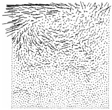
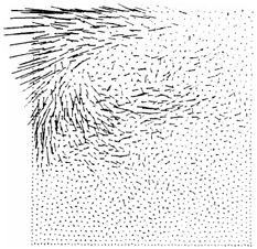
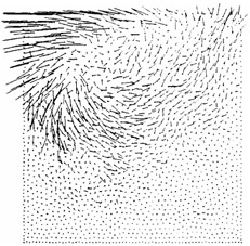
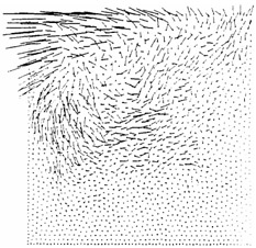
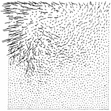
Consider now the cavity problem for the 1718 particles in Fig. 6.26. Let V = -1.0, ? T = 0.000002, J = 120000. Figures 6.27 6.30 show the resulting motion at the times T = 0.32, 0.64, 0.96, 1.28. Similar results were found for J = 160000, 80000, 40000. For clarity in the figures, the velocities were decreased by the factor mv = 0.021.
Example 1 is repeated with the change V = -2.0. Figures 6.31 6.34, at the respective times T = 0.32, 0.64, 0.96, 1.28, show the development of a primary vortex which is larger than the one developed in Example 1. Similar results were found for J = 160000, 80000, 40000.