6.11. Turbulence

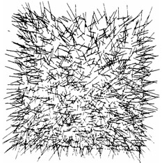
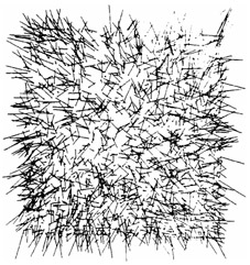
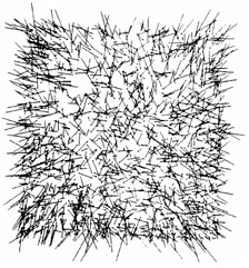
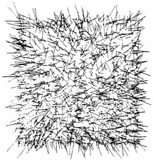
To simulate turbulence, set V = -20, ? T = 0.000001. Figures 6.39 6.42 show the flow development at T = 0.16, 0.32, 0.48, 0.64, for J = 40000. Each figure reveals the development of a strong current across the usual counterclockwise motion of primary vortices. For graphical clarity velocity vectors had to be decreased by the factor mv = 0.0055. Similar results followed for J = 160000, 120000, 80000.

Figure 6.39: V = -20, J = 40000, T = 0.16.

Figure 6.40: V = -20, J = 40000, T = 0.32.

Figure 6.41: V = -20, J = 40000, T = 0.48.

Figure 6.42: V = -20, J = 40000, T = 0.64.

Figure 6.43 shows an enlargement of the right portion of the flow in Fig. 6.42 in the region 0.11 < x < 0.125, and reveals the crosscurrent readily.

Figure 6.43: The section of Fig. 6.42 in the range 0.11 ? x ? 0.125.

Again, to support the contention that Figs. 6.39 6.42 represent fully turbulent flow, we now recall the definition of a small vortex. For 3 ? M ? 6,

we define a small vortex as a flow in which M molecules nearest to an ( M + 1)st molecule rotate either clockwise or counterclockwise about the ( M + 1)st molecule and, in addition, the ( M +...