2.8 The Gradient of a Scalar Function

Let f(x, y, z) be a real-valued differentiable function of x, y, and z, as shown in Figure 2.28. The differential change in f from point P to Q , from equation (2.47), can be written as

Figure 2.28: Illustration for defining gradient of scalar function

In terms of the differential length element

from P to Q, we can rewrite (2.69) as

or

where is a unit vector from P to Q in the direction of , and

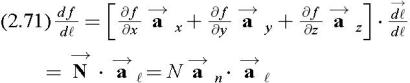
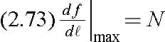
From (2.71) it is evident that the rate of change in the function f is maximum when _? and are collinear. That is,

There exists a surface passing through P on which f is constant. Similarly, there also exists a surface passing through Q on which f + df is constant. For the ratio df/d ? to be maximum, the distance d ? from P to Q must be minimum. In other words, df/d ? is maximum when _? is normal to the surface f( x, y, z) = constant. This, in turn, implies that is normal to the surface f( x, y, z) = constant. , by definition, is then the gradient of f( x, y, z). It is a common practice to write this gradient of f( x, y, z