2.1 Basic Concepts

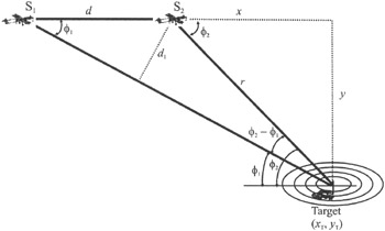
The geometry shown in Figure 2.1 can be used to describe the triangulation concept. Initially consider just two dimensions. There are two sensors, S ₁ and S ₂, separated by distance d, and a single target. Of course, the two sensors could be the same sensor that has moved distance d. Each of the sensors computes an LOB relative to some reference, which is the same for both sensors. By simple trigonometry,

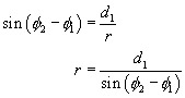
and

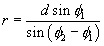
yielding

(2.1)

With knowledge of r and ? ₂, x and y, the distances to the target from S ₂, can be computed as

(2.2)

Figure 2.1: Geometric relationships for PF by triangulation.

These notions extend to more than two sensors and to three dimensions in the obvious way, taking two sensors at a time and computing the coordinates of the target. The resulting coordinates can then be averaged. Other methods of using more than two LOBs are discussed in this chapter.

Another technique for PF with triangulation is to plot (figuratively or literally) the measured LOBs and see where they cross, as shown in Figure 2.2 (the sensors could be one moving as shown or three stationary, and the same results would apply). In the absence of errors in the measurement process, these LOBs will all cross at a single point. However, in general, the LOBs are corrupted with measurement error and noise. This noise is frequently assumed to be zero mean additive white...