Electronic Warfare Target Location Methods

PF algorithms are presented in this section that are based on dynamic system models. These algorithms are typically applicable when the measurements are obtained recursively with the PF updated during each iteration. The section begins with a background discussion on dynamical systems before the algorithms are presented.
Dynamical systems can be described by the state transition equation:
| (2.115) | |
with s ? ? N and the measurement vector given by
| (2.116) | |
with z i ? ? p, where s i is the state of the system at time i and ? i is the state transition matrix, which can be linear, nonlinear, time variant, or time invariant. Matrix B relates the effects of the input u i-1 to the state s i at sample time i. The vector of random noise n i is usually modeled as white noise:
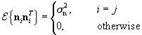
| (2.117) | |
| (2.118) | |
so
| (2.119) | |
where Q i is the covarance matrix of the process noise.
The measurement noise is characterized by
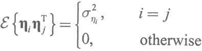
| (2.120) | |
| (2.121) | |
so
| (2.122) | |
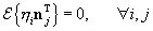
is the measurement error covariance matrix. The state variable noise and measurement noise levels are assumed to be independent:
| (2.123) | |
The N N matrix ? i relates the state at the previous time step i - 1 to the state at the current step i, in the absense of any driving function u i-1 or process noise n i -1.