2.2. Laplace Transform

Let us first state a few important points about the application of Laplace transform in solving differential equations (Fig. 2.1). After we have formulated a model in terms of a linear or a linearized differential equation, d y/dt = f( y), we can solve for y( t). Alternatively, we can transform the equation into an algebraic problem as represented by the function G( s) in the Laplace domain and solve for Y( s). The time-domain solution y( t) can be obtained with an inverse transform, but we rarely do so in control analysis.

Figure 2.1: Relationship between time domain and Laplace domain.

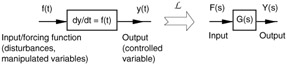
What we argue (of course it is true) is that the Laplace-domain function Y( s) must contain the same information as y( t). Likewise, the function G( s) must contain the same dynamic information as the original differential equation. We will see that the function G( s) can be "clean looking" if the differential equation has zero initial conditions. That is one of the reasons why we always pitch a control problem in terms of deviation variables. ^[4] We can now introduce the definition.

The Laplace transform of a function f ( t) is defined as

(2.4)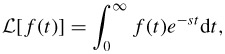

where s is the transform variable. ^[5] To complete our definition, we have the inverse transform,

(2.5)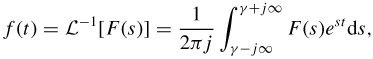

where ? is chosen such...