2.5. Partial-Fraction Expansion

Because we rely on a look-up table to do a reverse Laplace transform, we need the skill to reduce a complex function down to simpler parts that match our table. In theory, we should be able to "break up" a ratio of two polynomials in s into simpler partial fractions. If the polynomial in the denominator, p( s), is of an order higher than the numerator, q( s), we can derive ^[10]

(2.25)

where the order of p( s) is n and the a _i are the negative values of the roots of the equation p( s) = 0. We then perform the inverse transform term by term:

(2.26)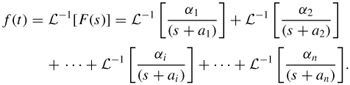

This approach works because of the linear property of the Laplace transform.

The next question is how to find the partial fractions in Eq. (2.25). One of the techniques is the so-called Heaviside expansion, a fairly straightforward algebraic method. Three important cases are illustrated with respect to the roots of the polynomial in the denominator: (1) distinct real roots, (2) complex-conjugate roots, and (3) multiple (or repeated) roots. In a given problem, we can have a combination of any of the above. Yes, we need to know how to do them all.