2.9. Linearization of Nonlinear Equations

Because a Laplace transform can be applied to only a linear differential equation, we must "fix" a nonlinear equation. The goal of control is to keep a process running at a specified condition (the steady state). For the most part, if we do a good job, the system should be only slightly perturbed from the steady state such that the dynamics of returning to the steady state is a first-order decay, i.e., a linear process. This is the cornerstone of classical control theory.

What we do is a freshmen calculus exercise in first-order Taylor series expansion about the steady state and reformulate the problem in terms of deviation variables. This is illustrated with one simple example. Consider the differential equation that models the liquid level h in a tank with cross-sectional area A:

(2.52)

The initial condition is h(0) = h _{s ,} the steady-state value. The inlet flow rate Q _in is a function of time. The outlet is modeled as a nonlinear function of the liquid level. Both the tank cross-section A and the coefficient ? are constants.

We next expand the nonlinear term about the steady-state value h _s (also our initial condition by choice) to provide ^[22]

(2.53)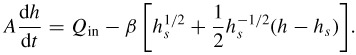

At steady state, we can write Eq. (2.52) as

(2.54)

where h _s is the steady-state solution and is the particular value of Q _in to maintain steady state. If we subtract the...