2.3. Laplace Transforms Common to Control Problems

We now derive the Laplace transform of functions common in control analysis.

1. Step function:

   (2.16)

   We first define the unit-step function (also called the Heaviside function in mathematics) and its Laplace transform ^[7]:

   (2.17)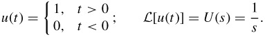

   The Laplace transform of the unit-step function (Fig. 2.3) is derived as follows:

   
   

   With the result for the unit step, we can see the results of the Laplace transform of any step function f( t) = Au( t):

   
   

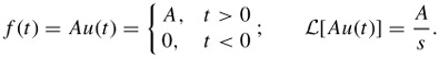
   The Laplace transform of a step function is essentially the same as that of a constant in Eq. (2.7). When we do the inverse transform of A/ s, which function we choose depends on the context of the problem. Generally, a constant is appropriate under most circumstances.

2. Dead-Time function (Fig. 2.3):

   (2.18)

   The dead-Time function is also called the time-delay, transport-lag, translated, or time-shift function (Fig. 2.3). It is defined such that an original function f( t) is "shifted" in time t ₀, and no matter what f( t) is, its value is set to zero for t < t ₀. This time-delay function can be written as

   
   

   The second form on the far right of the preceding equation is a more concise way of saying that the time-delay function f( t - t ₀) is defined such that it is zero for t < t ₀. We...