Radar System Analysis, Design and Simulation
The fast Fourier transform, forward and inverse, has found many applications in signal processing. Although the theory of fast Fourier transforms is well-known, numerous commercially available software packages have caused some confusion for beginners; some of them are written in radix 2, 4, or 8; in mixed radix 8 (4x2); decimation-in-time; or decimation-in-frequency scheme. Some codings are dedicated to real input/output only, others for complex input/output only, or sinusoidal input/output only, for example.
This chapter describes the basic building blocks of FFT and IFFT in radix 2 exclusively. The decimation-in-time and decimation-in-frequency algorithms will be explained in detail. All other algorithms readers may encounter are the variants of radix 2 of FFT and IFFT in order to shorten the computation time (to lessen the computation load) or minimize the memory size for certain specific applications.
The Fourier transform of a finite sequence is defined as
where
X[k]: Frequency sampled data;
x[n]: Time sampled data;
N: Total number of samples;
n: Time index, n=0, 1, 2, 3, ., N-1;
k: Freq index, k=0, 1, 2, 3, ., N-1.
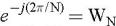
Using a shorthand notation,
Equation (4.1) and (4.2) can be written as,
When we examine (4.3) and (4.4), there is quite a large number of duplicated multiplications, and this adds operations. The FFT is an algorithm that eliminates the duplications by recognizing which indices "n" and "k" are repeated by what sequences. There are a few excellent textbooks that describe a rather simple concept but intricate steps to eliminate...