8.2 Derivation of Kalman Filter Equations
Refer to Figure 8.3. A passenger airliner has a smooth fight plan. The pilot plans to fly at a constant velocity at a constant altitude on a straight path. Due to non-constant engine thrust and nonuniform atmospheric conditions, the passenger airliner would traverse at varying velocities and an off-straight-line path.
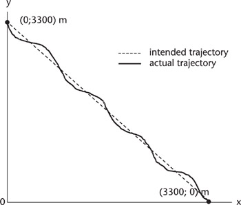 Figure 8.3: Flight trajectory
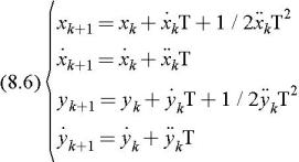
The position of the aircraft can be expressed in the Cartesian coordinate system (CCS) as follows. The overhead single dot ( ?) is velocity and two dots ( ??) acceleration. T is the discrete time measurement interval in seconds.
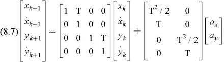
Recast the above Newtonian motion equations into a more compact form with a x and a y, representing accelerations in x and y axis.
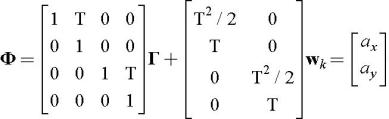
Equation (8.7) is still cumbersome. Can we write it the following vector-matrix form?
where
Equation (8.8) is the first of Kalman's seven equations and is called the state equation (the state of, or the position and the motion of, the passenger airliner).
The disturbance w k is assumed to be distributed as Gaussian with mean zero and variance ? 2. The covariance matrix Q k is given by,
We assumed that the accidental acceleration perturbations a x and a y at each measurement are completely uncorrelated and are small in magnitude, say 0.5g, uniformly distributed. (1g = 9.8 m/sec 2). (See Figure 8.4.) The expectation E{a xa y} is identically zero, for a x


 TABLE OF CONTENTS