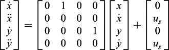
Up until now we have considered only a stationary receiver. Suppose the receiver was moving at a constant velocity. Let us try to apply extended Kalman filtering to the problem of tracking a moving receiver with two moving satellites. Now we are trying to estimate both the location and velocity of the receiver. It seems reasonable to make the receiver location and velocity states. If the receiver travels at constant velocity, that means the receiver acceleration (i.e., derivative of velocity) is zero. However, to protect ourselves in case the velocity is not constant we will include some process noise. Therefore, in our model of the real world, we will assume that the acceleration of the receiver is white noise or

where the same process noise u _s has been added in both channels. We can rewrite the preceding two scalar equations, representing our new model of the real world, in state-space form, yielding

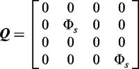
where u _s is white process noise with spectral density ? _s. The continuous process-noise matrix can be written by inspection of the linear state-space equation as

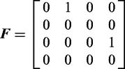
In addition, the systems dynamics matrix also can be written by inspection of the linear state-space equation as

Because F ² is zero, a two-term Taylor-series expansion can be used to exactly derive the fundamental matrix or

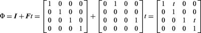
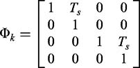
Substituting the sample time for time in the preceding expression yields the discrete fundamental matrix

The measurements are still the ranges...