Because we were successful in tracking the variable velocity receiver with an extended Kalman filter and two satellites, it is of considerable interest to see if we can be as successful with only one satellite. We have already demonstrated that the extended Kalman filter of Listing 11.8 was able to track a constant velocity receiver using only one satellite. Combining the same extended Kalman filter for the one-satellite problem (i.e., Listing 11.8) and the variable velocity receiver, we obtain Listing 11.10. The differences between this listing and Listing 11.8 (i.e., variable velocity receiver model) are highlighted in bold.

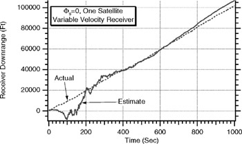
The nominal case of Listing 11.10 does not include process noise for the extended Kalman filter (i.e., ? _s = 0). This means that the filter is expecting a constant velocity receiver. We can see from Fig. 11.51 that having zero process noise does not cause the filter's estimate of the receiver location to diverge severely from the actual receiver location. However, we can see from Fig. 11.52 that the filter is not able to track the receiver velocity accurately. The filter is able to track the average velocity of the receiver, but it is not able to keep up with the velocity variations. These results are similar to those obtained with two satellites. However, when we only have one satellite, it takes much longer to get satisfactory estimates.

Figure 11.51: After a while the filter appears to be able to track receiver downrange location...