We have seen that the extended Kalman filter, using range measurements from two satellites, was able to track a receiver moving at constant velocity. The extended Kalman filter that was used did not even require process noise to keep track of the moving receiver. In this section we will see how the same extended Kalman filter behaves when the receiver is moving erratically.

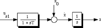
For our real world model we will still assume that the receiver is still traveling at constant altitude, but the velocity in the downrange direction will be variable. We will use a Gauss Markov model to represent the variable velocity. This is the same model (i.e., white noise through a low-pass filter) we simulated in Chapter 1. A block diagram of the model in the downrange direction appears in Fig. 11.36. Here we can see that white noise u _s1 with spectral density ? _s1 enters a low-pass filter with time constant T to form the random velocity. The time constant will determine the amount of correlation in the resulting noise. Larger values of the time constant will result in more correlation, and the resultant signal will look less noisy. The average value of the velocity is , which is added to the random component of the velocity to form the total velocity . The total velocity is integrated once to yield the new receiver downrange location x.

Figure 11.36: Gauss Markov model for downrange...