Intuitive Analog Circuit Design

In this chapter, the basics of signal processing and analysis are covered. The important tools offered in this chapter such as transfer functions in the Laplace domain, the concept of poles and zeros, step and impulse responses, and Bode plots are reviewed and needed by the reader in later chapters.
The transfer function and pole-zero plot of any linear time-invariant (LTI) system can be found by replacing all electronic components with their impedance expressed in the Laplace domain. For instance, the transformation from the circuit domain to the Laplace (or s) domain is made by making the following substitutions of circuit elements:
| Circuit domain | Laplace (s) domain |
|---|---|
| Resistance, R | R |
| Inductance L | Ls |
| Capacitance C | 1/ Cs |
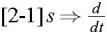
The resultant transformed circuit also expresses a differential equation; the differential equation can be found by making the substitution:
This transfer function of any lumped LTI system always works out to have polynomials in the Laplace [1] variable s. For instance, a typical transfer function with multiple poles and zeros has the form:
The values of s where the denominator of H(s) becomes zero are the poles of H(s), and the values of s where the numerator of H(s) becomes zero are the zeros of H(s). In this case, there are n zeros and m poles in the transfer function.
The values of s