Overview

Following Reference 1, consider the following testing integral

(D.1)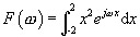

Integrating this yields

(D.2)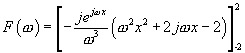

Thus the exact function can be expressed as

(D.3)

This was evaluated numerically using the conventional discrete Fourier transform (DFT) and fast Fourier transform (FFT) and then with the trapezoidal transforms, where

(D.4)

(D.5)

(D.6)

(D.7)

(D.8)

(D.9)

Here, N - 1 = 80 and M = 256. The DFT was evaluated as

(D.10)

The FFT was evaluated as

(D.11)

Some FFTs adopt the opposite sign convention. The trapezoidal DFT was evaluated as

(D.12)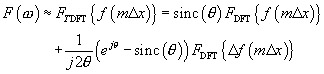

Either the DFT or FFT algorithm can be employed herein. Furthermore

(D.13)

(D.14)

In practice, the slope of the function is obtained by central differencing, whilst a right difference is taken at the left-hand side and a left difference is taken at the right-hand side, this can be expressed explicitly as follows

(D.15)

(D.16)

(D.17)

Results obtained from the DFT and the trapezoidal transforms can be found compared with the exact result in Figures D.1 and D.2.

Figure D.1: Comparison of exact and discrete rectangular transforms

Figure D.2: Comparison of exact and discrete trapezoidal transforms

Clearly, the first-order trapezoidal DFT offers a significant improvement over the more commonly employed zero-order rectangular DFT. A further comparison is made below in Table D.1. These values differ from those presented in the reference.