5.2 Alternative Forms

Consider first a planar surface y = 0. Following Karp and Karl (1965), a logical extension of the first order conditions (2.23) and (2.25) to the second order is

(5.1)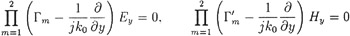

for some ? _m and , or equivalently

(5.2)

and although we can obviously choose a ₀ = = 1, it is more convenient not to do so. For the incident plane wave

(5.3)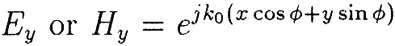

the corresponding reflection coefficients are

(5.4)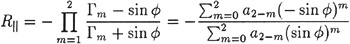

and

(5.5)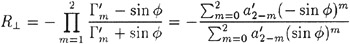

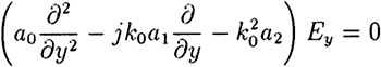
The boundary condition for E _y can be written as

where

(5.6)

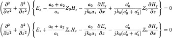
and using the wave equation we obtain

(5.7)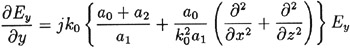

For the component H _y the analogous result is

(5.8)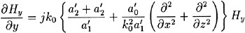

where

(5.9)

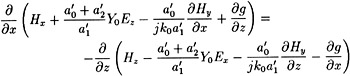
and now the only second derivatives are tangential ones. We can also express the conditions in terms of tangential field components. From Maxwell's equations and the fact that. ?. E = 0, (5.7) can be written as

(5.10)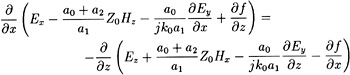

for any function f = f( x, z). Similarly, from (5.8),

for any function g = g( x, z), and therefore

(5.11)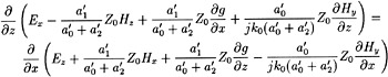

Choose

Then if

(5.12)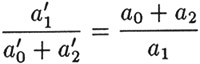

so that

(5.13)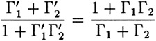

(5.10) and (5.11) imply

and by the same argument as that used in Section 2.3, we obtain

(5.14)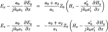

on y = 0+. Hence (Senior and Volakis, 1989)

(5.15)

which can also be written as

(5.16)

Provided the coefficients satisfy (5.12), the condition (5.15) is equivalent to (5.1) and, as the above analysis shows, can be obtained from (5.1) by a process of tangential...