6.1 The Root Locus An Introduction

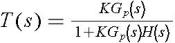
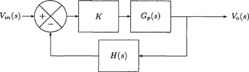
In this chapter we consider a third method of analyzing a system with feedback. We examine systems of the form shown in Figure 6.1. We consider the blocks G _p( s) and H( s) to be given and the gain, K, to be variable. Our goal is to plot the position of the roots of the denominator of the transfer function of the system:

Figure 6.1: The Typical System Analyzed by Means of Root Locus Techniques

with K as an implicit parameter. This is the plot of the system's poles and is called the root locus diagram ^[1] of the system. It gives us an idea of the effect of gain on the system's stability and performance. Often the gain, K, is not present in the physical system being analyzed. The virtual gain block is added to the system in order to understand the effect that additional gain would have on the system's stability and performance.

The System G _p( s) = 1/ s ², H( s) = 1 An Example

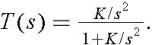
As we have seen G _p( s) = 1/ s ² is the transfer function of a simple satellite. We now analyze a system to control the angle of the satellite. We find that the transfer function of the system is:

We need to determine all of the roots of 1 + K/ s ². The solutions...