9.10 Biorthogonal Wavelets

When talking about wavelets, the transform is classified as either orthogonal, or biorthogonal. The previously discussed wavelet transforms (Haar and Daubechies) were both orthogonal. These can be normalized as well, such as by using 1/ ?2 and ?1/ ?2 instead of 1/2 and ?1/2 for the Haar coefficients. If you assume that we just take the square root of 1/2, you have missed a step. Instead, multiply by ?2, i.e., ?2(1/2) = ?2/2 = 1/ ?2. When it is both orthogonal and normal, we call it orthonormal.

The following structure (Figure 9.23) shows an example biorthogonal wavelet transform, and its inverse, for a single octave.

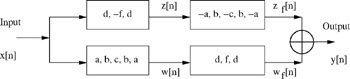Figure 9.23: Biorthogonal wavelet transform.

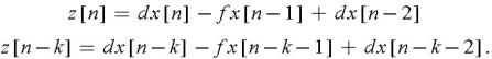
Proceeding as before, we start with definitions for w[ n] and z[ n]:

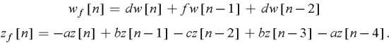
Now we can define w _f [ n] and z _f [ n] in terms of w[ n] and z[ n]:

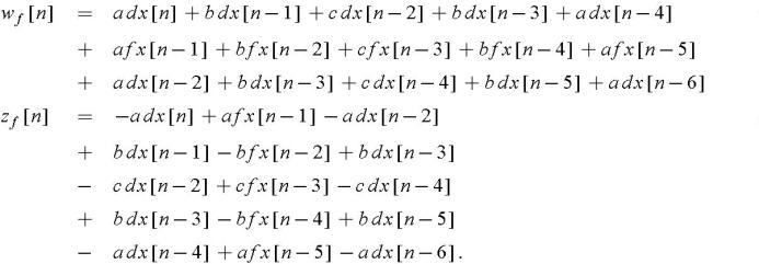
Next, we replace the z[ n]'s and w[ n]'s with their definitions:

These are added together to give us y[ n], the output:

Removing the terms that cancel, and simplifying, gives us:

To make y[ n] a delayed version of x[ n], we need the above expression to be in terms of only one index for x, that is, x[ n ? 3]. This can be accomplished if we...