5.3 Solutions of Ordinary Differential Equations (ODE)

A function y = f( x) is a solution of a differential equation if the latter is satisfied when y and its derivatives are replaced throughout by f( x) and its corresponding derivatives. Also, the initial conditions must be satisfied.

For example a solution of the differential equation

is

since y and its second derivative satisfy the given differential equation.

Any linear, time-invariant system can be described by an ODE which has the form

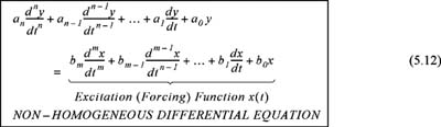
If the excitation in (B12) is not zero, that is, if x( t) ? 0, the ODE is called a non-homogeneous ODE. If x( t) = 0, it reduces to:

The differential equation of (5.13) above is called a homogeneous ODE and has n different linearly independent solutions denoted as y ₁( t), y ₂( t), y ₃( t),..., y _n( t).

We will now prove that the most general solution of (5.13) is:

where the subscript H on the left side is used to emphasize that this is the form of the solution of the homogeneous ODE and k ₁, k ₂, k ₃,..., k _n are arbitrary constants.

Proof:

Let us assume that y ₁( t) is a solution of (5.13); then by substitution,

A solution of the form k ₁y ₁(