5.7 Expressing Differential Equations in State Equation Form

A first order differential equation with constant coefficients has the form

In a second order differential equation the highest order is a second derivative.

An nth-order differential equation can be resolved to first-order simultaneous differential equations with a set of auxiliary variables called state variables. The resulting first-order differential equations are called state space equations, or simply state equations. The state variable method offers the advantage that it can also be used with non-linear and time-varying systems. However, our discussion will be limited to linear, time-invariant systems.

State equations can also be solved with numerical methods such as Taylor series and Runge-Kutta methods; these will be discussed in Chapter 9. The state variable method is best illustrated through several examples presented in this chapter.

Example 5.14

A system is described by the integro-differential equation

Differentiating both sides and dividing by L we get

or

Next, we define two state variables x ₁ and x ₂ such that

and

Then,

where ? _k denotes the derivative of the state variable x _k.

From (5.96) through (5.99), we obtain the state equations

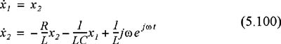
It is convenient and customary to express the state equations in matrix form. Thus, we write the state equations of (5.100) as

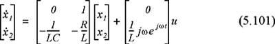
We usually write (5.101) in a compact form as

where

The output y( t) is expressed by the state equation

where C is another matrix, and d