4.6: Finite Difference Time-Domain Method in Three Dimensions
4.6 Finite Difference Time-Domain Method in Three Dimensions
Clearly the most general application of the FDTD, and the one of most interest in the calculation of RCS for realistic targets, is the three-dimensional formulation. The development of the update equations in three dimensions follows the same procedure as for one and two dimensions. The details have been worked out in several references.2 ,7
A three-dimensional Yee cell is shown in Fig. 4.39. As in the case for two-dimensions, we use the following shorthand notation:
-
Grid dimensions: ( ? x, ? y, ? z)
-
Time step: ? t
-
Nodes indices: (i, j, k) ? (i ? x, j ? y, k ? z)
-
Notation for field samples: E x (i ? x, j ? y, k ? z, n ? t) ? (i, j, k,)
Fig. 4.39: Yee cell for three-dimensional implementation of the FDTD.
The E components are defined in the middle of edges, whereas the B components are at the centers of the faces, denoted by integers plus one-half (for example i + 1/2). With this notation the magnetic field update equations are2
The electric field update equations are
where
and ? = x, y, or z. The three-dimensional formulation is the basis of several commercially available software packages.